Mathematical Discovery with Frontier Language Models: Progress, Practice, and Counterexample Search
Abstract
Frontier language models increasingly participate in mathematical research: solving difficult benchmark problems, proposing constructions, assisting proofs, and formalizing established arguments. Yet an impressive mathematical outcome is not a transparent measurement of the system that produced it. We survey progress through 19 September 2026, emphasizing the prompts, human interventions, search procedures, and verification practices behind reported achievements. We then examine the claim that frontier models prefer to falsify conjectures. A reproducible evidence supplement distinguishes assigned counterexample tasks, neutral strategy choice, verified solutions, and selected announcements, and codes bounded research cohorts by outcome, certificate, and workflow. The available evidence supports prompt dependence and some striking counterexample-oriented successes; it does not identify a general tactic preference. Constructive discoveries need not be refutations, and an asymptotic counterexample can require a substantial proof. We develop a conditional explanation based on model-specific verified utility, search opportunity, and verification and publication selection. Complete proofs establish utility-shift non-identifiability, a finite black-box certificate asymmetry, adaptive-search survival probabilities, attention-routing capacity, readout-sign neutrality, and verifier-induced amplification. These are explicit models and capacity results, not measurements of proprietary internals. Apparent counterexample preference must be decomposed into search, success, and observation before it is explained as a property of a model. We conclude with falsifiable experiments and a reporting protocol for human–AI mathematical discovery.
1. Introduction
Mathematical AI is moving from answering exercises to participating in research processes. The object being generated can be a numerical answer, a natural language argument, a search program, an extremal construction, or a formal proof. The surrounding process can be a single prompt, a mathematician’s extended conversation, an evolutionary search, or a coordinated collection of agents. These distinctions matter: the same final theorem can be reached by different combinations of human insight, model generation, computation, and verification. A survey that reports only which problem was solved loses much of what researchers need to understand or reproduce the achievement.
This paper follows the research process from problem choice to accepted result. It first surveys progress, then explains how people prompt and interact with models and how candidates are checked. It subsequently examines an intriguing claim: do frontier language models prefer to refute conjectures by counterexamples? A disproof is itself a proof, of the negation of the original statement. Our question concerns the choice and cost of a search route, not the mathematical legitimacy of refutation.
The question is motivated by the prominence of several constructive breakthroughs. Gowers’s discussion of the 2026 developments asks whether the relevant advantage is really counterexample finding, or instead a style of search that benefits from broad knowledge and many attempts [1]. A new object that improves a lower bound is not automatically a counterexample to an established conjecture; a counterexample to an asymptotic assertion may be an infinite family accompanied by a difficult argument. Nor does a final refutation show that a model began by looking for one. An unsuccessful proof search can reveal the construction, and a human can assign the disproof route in advance.
Several different questions are hidden in “preference.” Does the system choose counterexample search when alternatives are available? Is it better at constructing valid counterexamples than at producing matched affirmative proofs? Do its tools make constructions easier to check? Are refutations more likely to be selected, verified, or publicized? These are separate estimands. Our synthesis reports what the sources actually measure and leaves missing denominators visible.
Position. The public record does not yet identify a general frontier model preference for counterexamples. Apparent concentration in falsification should first be analyzed as the joint effect of the problem portfolio, prompting, model-specific search utility, verification, and reporting. Only a stable residual under controlled opportunities should be called a tactic preference. Conditional explanations of counterexample search are useful even when that stronger claim remains unestablished.
This position neither discounts a verified refutation nor predicts a permanent limitation of language models. False-theorem evaluations show that models can comply with demands for a proof even when a statement is false [2, 3]. Counterexample-specific tasks reveal difficulties in producing valid witnesses [4, 5]. An explanation must accommodate these failures as well as celebrated discoveries, and explain why changing the protocol could change the pattern.
Contributions and reading map.
We contribute four connected pieces. First, we organize recent progress by mathematical task and research workflow (Section 2, Section 3, Section 4, Section 5). Second, we provide an auditable extraction of published metrics and bounded discovery cohorts, preserving their different denominators (Section 6). Third, we connect operational definitions to complete mathematical derivations of search and selection effects (Section 7, Section 8). Fourth, we specify competing mechanisms and experiments that could distinguish a residual policy bias from opportunity and framing (Section 9, Section 10, Section 11). The supplement contains machine-readable records and code for the descriptive figures. No new frontier-model experiment is reported here.
Our intended audience is researchers in machine learning and mathematics. External mathematical results are summarized with their proof sources cited; the propositions used in our own explanatory argument are proved in full. The literature cutoff is a research snapshot, not a claim that systems or community judgments stopped changing on that date.
2. Scope, Sources, and Units of Evidence
2.1 What this survey includes
Our primary focus is frontier language-model systems used for mathematical problem solving and discovery during 2025–2026, with selected earlier work needed to explain their methods. “Frontier” is a dated description of the systems evaluated or reported as leading at the time of a study. It is not a single immutable set of models. We record the exact identifier when available and otherwise retain the source’s description, such as an internal reasoning model. We never infer that an unreleased system has the properties of a similarly named public model.
We include natural language proof generation, tool-assisted constructions, formal theorem proving, and autoformalization when they clarify the route from model output to mathematical knowledge. Short-answer benchmarks provide historical context; they are not substitutes for research validation. We do not attempt a complete history of automated deduction, educational applications, or all scientific uses of language models. Specialized systems are included as comparators when their search or verification mechanisms are relevant.
Two recent surveys already organize mathematical AI across informal reasoning, formal methods, and discovery [6, 7]. Our additional focus is the empirical and conceptual status of counterexample search: which outcomes can be counted, which process variables are observed, and what would be required to identify a preference. The bounded cohorts in Section 6 are not an exhaustive catalog of discoveries involving AI.
2.2 Search and extraction procedure
We searched primary publication venues and repositories, including arXiv, OpenReview, PMLR, the ACL Anthology, official research releases, benchmark organizers, and first-hand mathematical reports. Queries combined mathematical discovery, open conjectures, theorem proving, proof verification, human–AI interaction, counterexamples, prove-or-disprove evaluation, and named systems. Reference following from surveys and expert commentary supplied additional candidates; inclusion required a primary source for substantive claims. Search routes and retained sources are recorded in the supplement. This is a structured, targeted survey, not a claim of exhaustive database coverage or a registered systematic review.
The cutoff is 19 September 2026. We preserve the publication or revision version used for each numerical extraction and distinguish it from the access date. A newer paper can discuss an older experiment; a live benchmark can change its problem set or rubric. Such changes are part of the measurement, not incidental bibliographic details. Where reports give different counts, we retain the discrepancy and its context rather than silently combining them.
Eligible discovery records identify a mathematical target, an AI contribution, and an outcome. A result announcement without a checkable argument can be discussed as a claim, but it does not become verified through repetition. Reposts and duplicate releases do not add observations. Corrections remain attached to the original record. Unknown prompts, budgets, model versions, or failed-attempt counts are encoded as missing; absence of disclosure is not evidence of zero human intervention or a single attempt.
2.3 Three independent axes of classification
Outcome relative to the target.
An affirmation establishes the stated target; a refutation establishes its negation; partial progress improves a bound or resolves a restricted case; and unresolved means no accepted resolution is recorded under the stated protocol. The target must be specified before interpreting the outcome. Rewriting an existence theorem as the negation of an artificial universal does not turn it into a historically meaningful refutation.
Certificate and proof burden.
We separately code finite witnesses, construction families, existence arguments, general derivations, and mixtures. A finite object can require a long proof of its properties. A construction family can involve universal obligations over all sufficiently large sizes. “Constructive” and “cheap to verify” are not interchangeable. Classification follows the artifact, not the headline.
Workflow and attribution.
We distinguish autonomous attempts under a specified harness, human-guided sessions, externally assigned search directions, and formalization of existing mathematics. These categories describe a documented role, not a ranking of scientific merit. A human may choose the problem and verifier even when the subsequent search is autonomous. A model may make the decisive construction inside a collaborative session. We retain such contributions rather than forcing them into a binary human-versus-machine label.
2.4 Denominators and inferential scope
Relevant units include a distinct mathematical target, a model–problem attempt, an interaction session, and a released artifact. One target can generate many failed attempts and several successful artifacts. One announcement can contain multiple subresults. The tables state their unit; record-level details preserve these relationships. We deduplicate at the target or announced-entry level for discovery counts and retain separately reported repeated-run results as protocol-specific evidence.
The source cohorts differ in problem selection, truth status, tools, compute, and publication gates. We therefore avoid a pooled “counterexample rate” and a significance test against an arbitrary 50% baseline. Counts on a frozen collection describe that collection. Ambiguous classification is addressed through alternative codings; sampling intervals would require a sampling or repeated-trial design that the public record often lacks.
The extraction received a separate review for coding, denominator interpretation, and source consistency, documented in the supplement. These are agent-assisted audits, not independent human expert annotation. They improve traceability but cannot substitute for peer review of every external result. All aggregate figures are regenerated from the released data.
3. From Olympiad Medals to Research Claims
The period from 2025 through 19 September 2026 contains several genuine changes in what machine-assisted mathematics can do. It also contains several different kinds of achievement that are easily collapsed into a single story of “solving mathematics.” A score on unpublished problems with known answers is not a new theorem. A record construction is not a proof of optimality. Rediscovering a result missing from a database is not a novel resolution. Translating a known proof into Lean is not discovering that proof. Conversely, none of these distinctions makes the underlying achievement unimportant. They identify which capability has actually been demonstrated.
We therefore use five labels throughout this section. A benchmark solution answers a held-out problem whose solution is already known to the evaluators. A rediscovery independently recovers known mathematics. A bound or construction advance improves the literature without necessarily settling the associated extremal question. A research resolution proves or disproves a previously open statement. A formalization converts an informal statement or argument into a proof term checked by a kernel. The labels may overlap—a novel resolution can subsequently be formalized—but they should never be substituted for one another. We also distinguish a publicly accessible model from a public artifact produced by an unreleased model. A downloadable proof does not make the generating system reproducible.
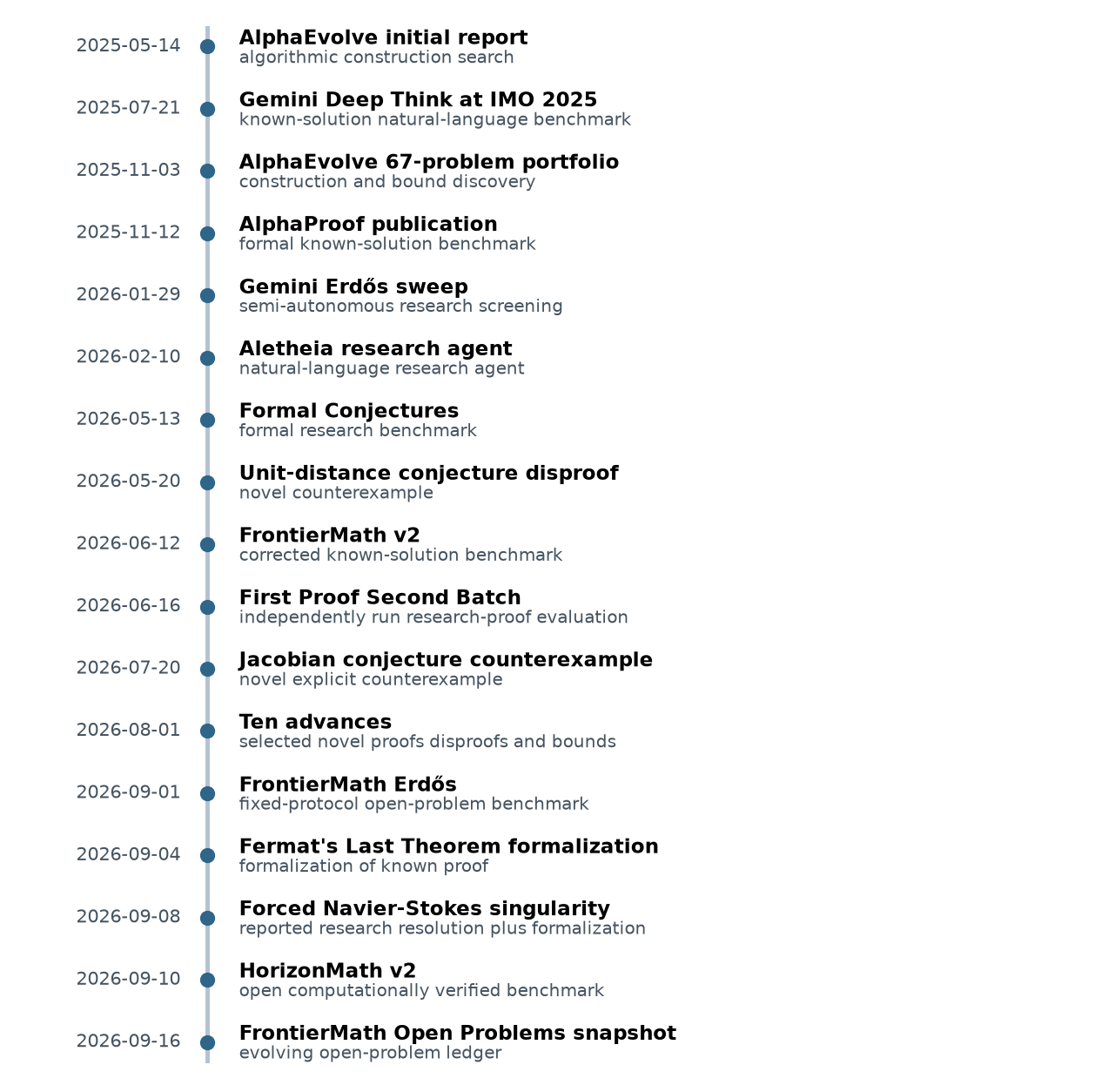
Figure 1. Dated progress timeline through 19 September 2026. Rows are ordered, not spaced by elapsed time. Dates denote public reports or designated snapshot revisions, not necessarily the day of discovery. Source details and numerical claims are in the text and the milestone ledger [8–24]. The Jacobian and Navier–Stokes entries are reported resolutions; publication, formal verification, and community acceptance remain distinct.
Three reporting variables are especially important when reading this timeline. The first is the sampling unit. A score may count a single model response, the best response after many restarts, a problem solved by at least one member of a system ensemble, or a selected result surviving expert review. These are different estimands. In particular, “seven problems had a passing solution” does not mean that each of four systems scored seven, and “five problems were solved at least once” does not describe a one-attempt benchmark. The second variable is the acceptance filter: automatic answer comparison, executable validation, a Lean kernel, blinded human referees, and later community uptake answer different questions. The third is the research boundary. If humans choose the target, formalize the statement, curate a library, redirect a search, select the best transcript, or rewrite the manuscript, the mathematical artifact may still be novel while the run is not end-to-end autonomous.
We consequently avoid a single cumulative “AI solved mathematics” count. Such a count would add unlike objects and amplify publication bias. A public benchmark normally exposes its failures and fixes a trial protocol; a company may reasonably publish only its most scientifically valuable internal successes. Both records are informative, but only the first estimates a rate under declared conditions. Similarly, availability has at least three levels: a public model or API, a reproducible harness around public models, and a public output from a private model. Several prominent late-2026 reports are in the third category. The proofs can be inspected even when the system that found them cannot be rerun.
3.1 The competition-to-research transition
AlphaProof provides the clearest prehistory. Its 2024 International Mathematical Olympiad result was published online in November 2025 and as a Nature article in 2026. AlphaProof solved three of the five non-geometry problems; combined with AlphaGeometry 2, the system solved four of six for 28 of 42 points, a silver-medal-equivalent score [11]. This was formal theorem proving: experts first translated the statements into Lean or another domain-specific language, the systems searched for checked proof objects, and experts translated the output back. The run used multi-day computation. The result demonstrated deep verified search on elite, known-solution problems, not autonomous reading or research discovery.
The next IMO result changed the interface. In July 2025 an advanced, unreleased Gemini Deep Think system received the official natural-language problem statements and returned natural-language proofs within the 4.5-hour contest limit. It solved five of six problems for 35 of 42 points. IMO coordinators graded the submitted solutions by the student rubric and certified the gold-medal-level score; their certification did not audit the model or experimental pipeline [9]. DeepMind describes parallel exploration, new reinforcement-learning methods, a curated corpus of high-quality solutions, and general Olympiad hints. This is a stronger demonstration of end-to-end mathematical communication than AlphaProof, but it remains a six-item competition evaluation using a special model whose exact search budget was not reported.
These two milestones matter because they separate three axes that later announcements often recombine: mathematical difficulty, autonomy of the language interface, and strength of verification. AlphaProof had kernel-level checking but human formalization and days of computation. Gemini had an end-to-end interface and contest-time output, but human grading. Neither by itself measures the chance of advancing an arbitrary research problem.
3.2 Search over constructions: AlphaEvolve
AlphaEvolve illustrates a different route. It represents a candidate construction as code, uses Gemini models to propose mutations, runs an automatic evaluator, and retains promising programs in an evolutionary loop [8]. The initial May 2025 report said that the system was applied to more than 50 open problems: it rediscovered a state-of-the-art solution in roughly 75% of cases and improved the best-known solution in 20%, according to the authors. Examples included a 48-scalar- multiplication algorithm for multiplying complex matrices and a 593-sphere construction giving a new lower bound for the eleven-dimensional kissing number.
A later, more transparent mathematical portfolio studied 67 solved and unsolved problems across analysis, combinatorics, geometry, and number theory [10]. It reports matching the best known result in most cases, improvements in several, failures as well as successes, and some experiments in which Deep Think or AlphaProof helped turn a finite construction into an argument. The repository publishes problem descriptions and many prompts, evaluators, initial programs, and evolved outputs, but not the AlphaEvolve service itself. Importantly, the earlier 75% and 20% figures were stated for “over 50” open problems and must not be presented as fractions of the later 67-problem portfolio. This work supports a capability for verifier-friendly construction and bound search. It does not establish a comparable ability to prove upper bounds over all possible constructions.
3.3 Research agents and independently run proof evaluations
DeepMind’s Aletheia system moves from program evolution to long-horizon natural-language research. It repeatedly generates, critiques, and revises candidate arguments using an advanced Gemini Deep Think model and search tools. The accompanying report separates an AI-generated arithmetic-geometry paper, a human–AI collaboration, and a semi-autonomous sweep of Erdős problems, and proposes explicit autonomy and interaction records [13]. This taxonomy is more informative than the single word “autonomous”: humans still select questions, supply infrastructure, audit novelty, and decide which outputs become papers.
The Erdős sweep supplies an unusually useful denominator: 700 entries marked open in Bloom’s database. The version-3 report distinguishes four seemingly novel results from nine prior-solution cases, with partial results among the former [12]. Earlier versions differed. Section 6 preserves the coding and selection stages. The key lesson for research evaluation is that correctness, fidelity to the intended statement, and novelty require separate audits.
First Proof’s second batch adds independent evaluation. Organizers ran four systems on ten unpublished, already-solved research problems under a 24-hour, no-follow-up protocol. A technical failure left 39 submissions; 30 domain experts supplied double-blind reviews. Across the union of systems, seven problems received a passing solution and two more an approach needing major revision [17]. This is not a seven-out-of-ten score for any single model. The organizers required code and logs, enabling closer inspection of the workflow than an internal showcase permits. The first February batch was an informal, ungraded public experiment and should not be merged with this evaluation.
3.4 Benchmarks designed around the research frontier
The benchmark landscape itself changed quickly. FrontierMath Tiers 1–4 contains hard but solved, automatically scored questions. Its June 2026 v2 release addressed errors in 42% of items, including removals, and left 338 problems: 295 in Tiers 1–3 and 43 in Tier 4 [16]. Consequently, scores on the older 180-, 300-, or 350-item versions are not interchangeable with v2. The task asks for a closed-form answer through a Python-enabled interface, so a correct score demonstrates problem solving but not a human-readable proof. OpenAI funded the original dataset and has access to much of it, with defined holdouts; that conflict and the version must accompany reported scores.
FrontierMath: Open Problems instead tracks unsolved questions equipped with bespoke executable verifiers. As of 19 September, its page listed 49 active problems: 41 unsolved, four classified as solved by AI, and four as solved by human–AI collaboration [24]. This is not an model score. Problems, access, attempts, and attribution vary; failed attempts stopped being displayed in June; and the site introduced the human–AI category only on 16 September. The evolving ledger is valuable precisely because it records construction, counterexample, record, and notability labels rather than forcing all progress into one accuracy number.
Two open resources cover different verification regimes. Formal Conjectures reported 2,615 Lean statements in May 2026, including 1,029 open research conjectures and 836 solved problems suitable for autoformalization evaluation [14]. A successful proof there is kernel-checkable, subject to the separate risk that the formal statement misrepresents its informal source. HorizonMath v2 contains 113 predominantly unsolved, computationally verifiable problems in eight domains. Its September revision reports six novel improvements or resolutions, three each from GPT-5.4 Pro and GPT-5.6 Sol, while most evaluated systems scored below 10% [23]. These benchmarks exploit a generator–verifier gap: discovering an object may be difficult even when checking it is cheap. They consequently sample only the portion of research mathematics admitting such certificates.
FrontierMath Erdős instead evaluates prominent open statements in Lean. Its fixed set has 68 conjecture statements from 65 Erdős problem numbers. Five systems received one attempt per statement with a $300 and 72-hour cap; only prerelease GPT-6 Astra solved any, producing one proof and one disproof [20]. Nonuniform repeat search increased the distinct solved set to five. Section 6 separates those protocols and their denominators. The experiment illustrates a demanding research boundary: discovery must be followed by formalization, and the formal statement itself still needs expert scrutiny.
3.5 Reported research resolutions, May–September 2026
In May, an internal OpenAI model generated a counterexample to the Erdős unit-distance conjecture, giving an infinite family with polynomially more unit distances than the conjectured order. Nine mathematicians published a digested, human-verified account [15]; OpenAI described the underlying system as a general-purpose reasoning model tested on a wider collection of Erdős problems [25]. The result is a research disproof, but the collection size, number of attempts, search budget, and failures were not disclosed. It is therefore evidence of capability, not an empirical success probability.
July brought an especially compact claimed counterexample to the general Jacobian conjecture: an explicit polynomial map on with constant nonzero Jacobian and a displayed collision. A short mathematical manuscript verifies the example and its higher-dimensional stabilization, while Anthropic later attributed the resolution to Claude Fable 5 [18, 26]. The algebraic certificate is short and independently checkable, while the discovery record is sparse: the original public evidence did not include a full transcript, budget, or controlled protocol. The result leaves the two-variable case open. It belongs in a survey of checkable AI-assisted discoveries, but not in a benchmark numerator without a denominator.
On 1 August, OpenAI released manuscripts for ten selected advances spanning sphere packing, coding theory, group theory, operator algebras, circuit and quantum complexity, lattice hardness, geometry, and extremal combinatorics [19]. OpenAI attributes the mathematical arguments to an internal Astra version and estimates that solution-finding tokens would cost about $2,000 at Sol API rates. Humans and the model prepared the manuscripts; the model then produced public Lean certificates. Some entries are full resolutions, some disproofs, and some improved bounds. The release does not report how many problems or attempts were screened, so “ten advances” is a selected portfolio, not ten successes out of ten trials.
Anthropic’s 4 September Fermat’s Last Theorem release is a different category. Dozens of agents using a Claude Code harness and Prove2Me reportedly spent 11 days and about six billion output tokens producing 13 million lines of Lean. The final development proved 30,300 intermediate theorems, using about 29,500, and was checked by Lean, Comparator, and an independently implemented Lean kernel documented in the released repository [21]. Tianyi Peng supplied occasional high-level priorities, and Kevin Buzzard reviewed the artifact. This is an extraordinary formalization of the established Frey–Serre–Ribet–Wiles–Taylor–Wiles argument, not a new proof of an open conjecture. Its scale also shows why “short informal proof” and “machine certificate” are not comparable cost units.
Finally, on 8 September OpenAI reported a finite-time singularity for forced three-dimensional Navier–Stokes, corresponding to alternatives C and D in the Clay formulation on and the torus [22]. The internal model was described as more capable than GPT-6 Astra. Separate groups explored proof and disproof variants; the group producing the reported solution involved roughly 10,000 concurrent agents. Humans redirected resources after a related Euler result and cross-pollinated agent groups. OpenAI reports 88 hours to the argument, 17 further hours for Astra to formalize it, and roughly 130 billion output tokens for the Navier–Stokes effort. The paper and Lean artifact are public, but as of 19 September the result was too recent for settled community acceptance; OpenAI explicitly declined to claim the prize. It should be described as a reported, formally certified forced-case resolution pending broad mathematical review, not silently substituted for the better-known unforced question.
3.6 What the record supports
The record now supports three restrained conclusions. First, frontier systems can produce some novel, checkable mathematics: this is no longer inferred only from benchmark extrapolation. Second, many documented workflows deliberately provide a crisp verifier—Lean kernels, executable evaluators, explicit constructions, or short algebraic witnesses—so the record is enriched for problems with cheap checking; it does not estimate how success varies with verifier availability. Third, the public evidence remains poorly calibrated. The best controlled studies show low or union-of-systems rates, whereas the most dramatic internal-model announcements omit denominators.
Nothing in this chronology by itself establishes a general preference for counterexamples. The fixed FrontierMath Erdős run produced one proof and one disproof; its expanded runs produced three proofs and two disproofs. AlphaEvolve is structurally aimed at constructions, and headline selection may favor memorable refutations. The appropriate conclusion is thus about an emerging capability and an evaluation asymmetry, not an intrinsic tactic preference. Measuring the latter requires the matched, preregistered design developed in the rest of this paper.
4. How People and Models Conduct Mathematical Research
A research workflow is more than a prompt. It specifies how questions are selected, which information is available, how candidates are generated, who interprets failures, and when a result is accepted. This section organizes those choices into reusable patterns. The examples are documented procedures, not recipes guaranteed to reproduce the original discoveries on today’s public models. We distinguish a prompt released with an experiment from a prompt reconstructed after success, and both from our own illustrative templates.
4.1 A shared description of interaction
Let a research state at step be
where is the current target, the accepted lemmas, the unresolved candidates, the recorded evidence, and the remaining resource budget. A model proposes an action : derive a lemma, construct an object, retrieve a reference, run code, request a check, or abandon a branch. A verifier returns feedback , and a human may supply intervention . The state update
is a description of the workflow, not a claim about the model’s internal representation. It highlights why independent sampling from a fixed candidate distribution is often inappropriate. Failed checks, new lemmas, and human judgments change subsequent search.
A useful research log preserves the proposed action, the returned evidence, and the resulting change in state. A polished final proof suppresses most of this information. It may reveal the certificate but not the search that found it. An abridged reasoning trace also need not expose the allocation of hidden computation. We therefore treat visible traces as observations of a communication channel, with the limitations established by work on unfaithful explanations [27].
Table 1. Documented workflow patterns. Model roles, source URLs, and the complete extraction are in the supplement. These are examples, not controlled comparisons of workflow effectiveness.
| Workflow / example | Human contribution | Feedback | Interpretation |
|---|---|---|---|
| Direct resolution Unit-distance report[25] | Target selection; expert exposition and checking | Expert mathematical review | Selected success; trial denominator unknown |
| Interactive repair Nesterov convergence[28] | Filter claims; consolidate facts; transfer continuous-time proof | Human rejection and lemma repair | Human-guided affirmative discovery |
| Program evolution AlphaEvolve[10] | Define target; design evaluator | Executable score and constraint checks | Construction or bound search |
| Research agent Aletheia[13] | Choose problems; review outputs and novelty | Model critique plus tools | Harness-specific research process |
| Formal proof search AlphaProof[11] | Formalize statements; configure task | Proof-assistant checking | Known-solution benchmark; verified derivations |
| Coordinated agents Navier-Stokes report[22] | Allocate routes and resources; share intermediate results | Inter-agent work and formalization | Terminal route is not spontaneous initial choice |
4.2 Direct resolution and portfolios
The simplest interface gives a precise statement and requests a resolution. For an unknown conjecture, neutral wording permits both proof and refutation. For a known theorem, a request to reproduce or formalize its proof has a different purpose. Asking for a counterexample on every task is an intervention on strategy, not a neutral measurement of what the model would choose.
The unit-distance report is a useful direct-resolution case. Its released problem prompt asked for either an affirmative or negative resolution. An accepted response was subsequently rewritten and examined by mathematicians; the expert companion clarifies and contextualizes the argument [25, 15]. The report does not disclose the failed-attempt denominator. Consequently, a successful individual response and a successful portfolio are not equivalent claims.
Portfolio search repeats a task across seeds, models, or prompt variations and then selects candidates. Selection can occur through answer voting, an independent judge, code, or expert scrutiny. Training and inference studies show how verifiers and additional computation can improve mathematical performance [29–31]. But reporting only the selected transcript hides the cost of the discarded candidates. For research claims, the relevant account includes every attempted problem and the stopping rule, even when full traces cannot be released.
A practical direct-resolution prompt should specify the domain, quantifiers, allowed assumptions, expected certificate, tools, and permitted uncertainty. It should ask the model to identify any unproved lemma it uses. These are reporting recommendations, not measured universal improvements in accuracy.
4.3 Human criticism, consolidation, and transfer
Human interaction can change the search distribution much more than a small prompt paraphrase. A mathematician decides which partial results survive, which failed approaches deserve repair, and which apparent reductions simply rename the difficulty. These interventions should be recorded as mathematical contributions rather than hidden behind the final model response.
Jang and Ryu’s Nesterov-convergence work documents this process. Using GPT-5 Pro, they estimated that about 80% of proposed arguments were incorrect. They filtered and consolidated the useful ideas, then supplied a continuous-time proof in LaTeX to guide the discrete-time argument. A later one-shot prompt succeeded on its third trial; this retrospective success did not reproduce the original interactive discovery [28]. This case illustrates both a new affirmative proof and the importance of human branch management.
Another mode gives the model a tightly specified intermediate lemma. In OpenAI’s early science report, Gowers tested a compactness subproblem and checked the proposed application of a known theorem; later interaction exposed remaining mismatches between the local statement and the intended larger argument [32]. Solving a local lemma is valuable, but its usefulness depends on its hypotheses and on the unresolved obligations connecting it to the main theorem.
We recommend maintaining a distinction between accepted facts, promising conjectures, and rejected claims in a session. If all three are compressed into a natural-language summary without labels, a later model can treat a speculative step as established. A compact proof-state ledger should retain the exact statement, assumptions, provenance, and reason for acceptance. This is also essential for measuring tactic switching: a session that begins with a proof attempt can end with a counterexample suggested by the failed lemma, and the reverse can occur.
4.4 Program-guided construction and generalization
In an evaluator-guided workflow, the model generates or modifies a program that proposes mathematical objects. An external evaluator checks constraints and scores a target quantity. Search can then improve the program, the object, or both. The role of the human is often concentrated in designing the evaluator and deciding whether its score captures the intended mathematics.
The later AlphaEvolve study releases many problem formulations and evaluator artifacts, including unsuccessful explorations. Its finite-field construction work shows a further transition: numerical or finite examples can motivate a parametric construction and then a proof [10]. These are distinct deliverables. A program that succeeds for tested sizes is not yet a theorem for all sizes; a proof must explain why the construction continues to satisfy every required property.
Consider, as a generic example rather than a reported experiment, a search for a graph with many edges and no forbidden subgraph . A candidate graph can be represented by an adjacency matrix, checked exactly for forbidden copies, and scored by its edge count. A better score proves a lower bound for the extremal function at that size. It does not prove an upper bound, nor does it necessarily refute any particular conjecture. The original target and its quantifiers determine the outcome label.
Such workflows make some construction tasks especially accessible because failure returns structured information: a violating edge pair, an inadmissible parameter, or a concrete execution trace. A general proof can also admit structured feedback through a proof assistant. The relevant distinction is the available feedback channel and certificate burden, not simply whether the final prose says “proof” or “counterexample.”
4.5 Generator–verifier loops and formal pipelines
A natural-language research agent can alternate between proposing an argument, criticizing it, and revising it. Aletheia makes these roles explicit and releases interaction material alongside its research reports [13]. A judge model is useful for triage, but correlated errors can survive both generation and criticism. Self-consistency across several agents is not a substitute for a check of the mathematical statement.
Formal pipelines replace at least part of that feedback with a trusted proof checker. AlphaProof combines proof search and reinforcement learning with formal checking; its IMO experiment also used candidate-answer filtering [11]. A failed candidate can be eliminated before expensive proof search, but the filtering protocol itself shapes which routes receive resources. This is a concrete motivation for the verifier-amplification model developed later, rather than evidence that its simplified assumptions hold quantitatively in that system.
Formalization introduces its own research state: definitions, lemma dependencies, library coverage, and unresolved goals. Repeatedly sending the entire project to a model can waste context and obscure dependency errors. A dependency graph makes it possible to assign a local goal together with the precise statements of its prerequisites. The reported Fermat formalization used such a structure through Prove2Me [21]. This illustrates organizational support for long arguments, separate from discovering a new mathematical idea.
4.6 Coordinated agents and externally chosen routes
Parallel agents can explore independent guesses, work on separate lemmas, or exchange results. These arrangements have different statistical implications. Independent attempts can estimate a pass rate under a fixed protocol; agents that share discoveries are dependent parts of one adaptive search. Counting them as independent successes would exaggerate evidence.
The Navier–Stokes report explicitly assigned affirmative and negative variants to different groups, followed by resource reallocation and exchange of intermediate results [22]. Its terminal disproof therefore cannot identify a spontaneous initial tactic choice. The choice of the successful route was partly an experimental design and partly a selection outcome.
For collaborative research, an interaction record should include who supplied each reduction, which agents could communicate, what was shared, whether the model changed during the run, and what prompted termination. Costs should include rejected candidates and downstream verification, not just the final response. These records make it possible to distinguish a model’s behavior from the behavior of the larger research system.
4.7 From workflow descriptions to testable comparisons
A workflow can change capability without changing a latent preference. Providing a missing lemma can increase proof success. Adding an executable checker can make counterexample search productive. A prompt demanding a proof can suppress rejection of a false premise. Each change affects an observed rate through a different path.
The survey therefore uses case studies to identify variables and failure modes, not to rank workflows causally. A comparison of two published successes cannot tell us what would have happened under swapped prompts, equal compute, or the same verifier. Randomized comparisons are needed for that purpose. Until then, the most useful practical questions are concrete: what did the system receive, what did it try, what feedback changed the next step, and what exactly was checked at the end?
5. Verification, Novelty, and Acceptance
A mathematical result has several distinct burdens: the proposed artifact must be valid, it must address the intended statement, and its claimed novelty must survive comparison with the literature. Formal verification strengthens one part of this chain. It does not by itself settle all three. We use a verification matrix rather than a single ladder in which every formal artifact is assumed to dominate every human assessment.
5.1 What different checks establish
Table 2. Verification channels and the claims they can support. No row alone establishes novelty, attribution, and faithful problem formulation.
| Channel | Evidence supplied | Principal remaining obligation |
|---|---|---|
| Model critique | A candidate error or alternative argument | The critique may share the generator’s error |
| Numerical experiment | Behavior at tested parameters and precision | Exactness, generalization, and untested cases |
| Executable checker | Satisfaction of encoded finite constraints | Checker correctness and correspondence to the target |
| Symbolic calculation | Exact identities in a declared algebraic setting | Side conditions, domains, and full proof context |
| Proof-assistant kernel | A derivation of the encoded proposition | Statement alignment, axioms, dependencies, implementation |
| Expert review | Assessment of argument, context, and relevance | Residual error and incomplete specialist coverage |
| Literature audit | Evidence concerning priority and novelty | Coverage, terminology changes, inaccessible sources |
An executable counterexample checker should test both admissibility and failure of the conclusion. If a purported counterexample violates a premise, it is not a refutation. For a numerical search, tolerances must be justified: floating-point proximity to an equality is not an exact algebraic identity. A symbolic simplification must use the correct domain and side conditions. An interval or exact-arithmetic certificate can close some of these gaps, but the mathematical interpretation of the code still needs review.
The same care applies to affirmative arguments. A model can establish a lemma correctly and invoke it where its assumptions fail. It can cite a real theorem with a subtly stronger conclusion than the original. A checker limited to the final numerical answer may not detect either problem. Conversely, a flawed exposition can contain a recoverable central idea. Evaluation should say whether it accepts only complete proofs or also arguments requiring repair.
5.2 Formal statement fidelity
Let be the intended mathematical claim and the proposition given to a proof assistant. Kernel acceptance supports a judgment of the form
where contains the definitions and permitted axioms. The separate translation obligation is that this proposition faithfully expresses . A checked theorem about a weakened hypothesis, a finite truncation, or an altered definition does not automatically solve the original problem. This is a distinction between two claims, not a criticism of formal logic.
For a released formal artifact, the record should identify the theorem, dependencies, checker version, and admitted axioms. Review should exclude unproved placeholders and confirm that the checked endpoint is the advertised statement. If a tactic uses external computation, its certificate and trust assumptions must be visible. An independent checker reduces reliance on a single implementation, while independent statement review addresses a different risk.
Formal Conjectures makes statement curation and revision part of the benchmark itself [14]. FrontierMath Erdős likewise notes that some newly generated formalizations had received only initial review at release [20]. These details should travel with a performance number. Formal verification can be rigorous while the connection to the intended informal problem remains under examination.
5.3 Human review and correction
Expert review does more than assign a binary score. A specialist can recognize a hidden assumption, identify a known result in unfamiliar notation, shorten a proof, or clarify the significance of a construction. Such contributions may occur after the initial AI output and should be distinguished from the discovery transcript. A human-readable exposition also helps other mathematicians reuse a result whose formal certificate is too large to inspect directly.
The Nesterov-convergence paper supplies a particularly useful correction. Its revised version withdraws earlier partial results for damping parameters , attributing the error to insufficient checking of model-generated arguments [28]. The correction concerns that extension, not a blanket retraction of the principal convergence result. Keeping the version history prevents the survey from counting a removed claim as current evidence.
First Proof’s second batch used multiple domain referees and distinguished minor from major revisions [17]. This makes its judgments more informative than a single automatic score, but they should still be quoted using the organizers’ acceptance categories. A report that groups repairable arguments with complete proofs must not be compared directly with a kernel-only benchmark without explaining the changed criterion.
5.4 Novelty is a separate search problem
Correctness does not establish novelty. An apparently open database entry may already have a solution under another name; a model may retrieve an argument without identifying its source. In the Gemini Erdős sweep, several addressed entries were resolved through literature identification rather than new mathematics [12]. The resulting contribution can be useful, but it belongs in a different category from a new theorem.
A novelty audit should search alternative formulations, stronger prior results, related constructions, and the references of any theorem invoked. It should also record the model’s access to browsing and supplied papers. After a result is published, rerunning a prompt may retrieve it, so a successful later run does not reproduce the original discovery. A dated problem snapshot and archived pre-solution interaction help, but no public transcript alone reveals every possible training-data overlap.
We therefore track novelty status separately from verification status. “Reported new,” “independently assessed as new,” “rediscovered,” and “uncertain” are not interchangeable. Nor is expert recognition of importance equivalent to verification of every proof step. Recent announcements may have strong formal artifacts while their interpretation and community assessment remain in progress.
5.5 Verification effort and observed selection
The cost of a research result includes discovery, checking, repair, formalization, and exposition. A short output can require substantial expert work; a long formal artifact can have a cheap final kernel check but expensive construction and statement review. These quantities should not be collapsed into generated-token count.
This matters for counterexample statistics. If explicit finite objects are easier for a reviewer to check than long general arguments, they may reach the public record more quickly even when the generator attempts both equally. Conversely, a counterexample requiring a delicate asymptotic analysis may receive no such advantage. The relevant quantities are the actual certificate and review costs under the chosen system.
The flow from candidate to published mathematics therefore contains several filters: validity, fidelity to the question, novelty, significance, and editorial selection. A statistic conditioned on the final filter cannot recover earlier tactic allocation without additional information. The selection model in Section 8 makes this observation precise. It also explains why a survey should retain unresolved cases and corrections rather than treat them as inconvenient noise.
6. Quantitative Evidence on Counterexample Use
6.1 Four different empirical questions
A preference is a property of a decision rule under specified alternatives, not a synonym for a successful disproof. We distinguish four observable quantities: the strategy selected before feedback; performance when falsification is assigned; the mathematical direction of accepted results; and the composition of publicly reported discoveries. Only the first directly measures strategy choice, and even it requires matched opportunities and utilities. The other three are informative about mathematical practice but mix task selection, ability, verification, interaction, and reporting.
We therefore report four bounded cohorts rather than assemble a leaderboard of famous counterexamples. Table 3 separates the fixed and expanded FrontierMath Erdős protocols; Figure 2 displays positive-result composition without pooling cohorts. Each discovery record has a directional code, a resolution-status code, a certificate code, and a workflow code. An affirmative construction is not automatically a refutation. Partial progress is not a complete solution. A proof that a counterexample cannot exist is not coded as a successful counterexample merely because the original task requested one. The supplement preserves these distinctions and the sources needed to challenge them.
Table 3. Separate bounded cohorts. A = affirmative result, R = refutation, O = mixed/other; the target and scope qualifications in the text are essential. The addressed column includes partial and literature-based Gemini results. The two Erdős rows overlap and must not be added.
| Cohort | Total | Addressed | A | R | O |
|---|---|---|---|---|---|
| Gemini Erdős v3 | 700 | 13 | 6 | 6 | 1 |
| OpenAI selected ten | 10 | 10 | 7 | 3 | 0 |
| Erdős fixed Astra | 68 | 2 | 1 | 1 | 0 |
| Erdős all Astra attempts | 68 | 5 | 3 | 2 | 0 |
| Open registry (19 Sep.) | 49 | 8 | 1 | 0 | 7 |
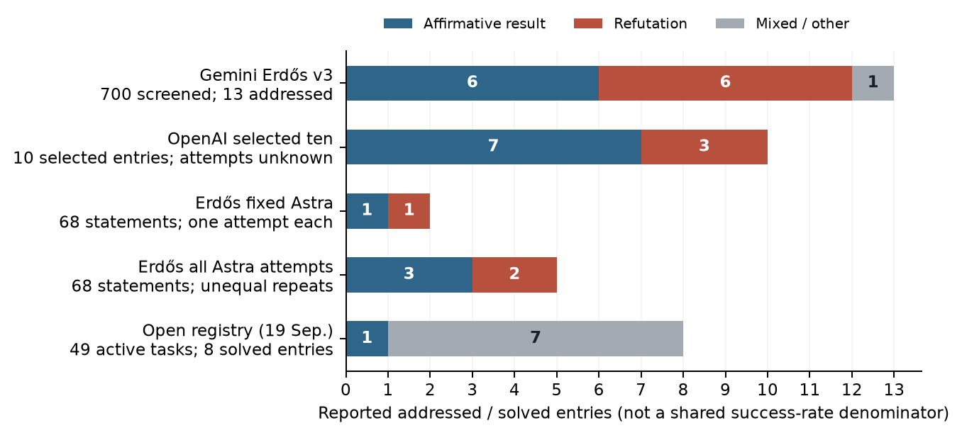
Figure 2. Directional classifications of positive entries within separately bounded cohorts. Row labels state the originating cohort; bar widths count positive entries, not interchangeable trials. The Gemini cohort includes partial answers and prior-literature resolutions; OpenAI’s collection is selected; the two Erdős rows overlap; the registry mixes systems and workflows. These bars do not estimate an intrinsic preference.
6.2 The bounded discovery census
Gemini’s 700-problem deployment.
The version-3 full text of [12] reports 13 meaningfully addressed problems from 700 inputs: two full and two partial apparently novel answers, four rediscoveries, and five literature identifications. The paper’s PDF inventory takes precedence over a stale landing-page abstract that still says five novel and eight prior results. Our directional coding is six affirmative, six negative, and one open-ended resolution. Thus describes negative directions among positive entries, not novel counterexamples among 700 attempts. Coding the limit evaluation in problem 1089 as an affirmative answer instead gives seven affirmative and six negative entries. Of the four apparently novel entries, two are affirmative and two are partial negative answers. Problem 654 needs a parameterized construction, not merely one finite test. The 13 records include expert corrections and rewritten explanations; we retain their stated verification status rather than treating raw model text as final mathematics. The model was Aletheia on the November 2025 Gemini Deep Think base.
OpenAI’s ten announced advances.
The collection supplies a complete showcase denominator, not a complete attempt denominator [19]. We count each of its ten numbered entries once. In the 6 August manuscript, entries 3, 4, and 10 refute universal claims; entry 10 contains two separate disproofs but remains one showcase entry. The narrow result is therefore , with seven affirmative theorems. Counting the Ramsey construction in entry 9 as a counterexample to a finite-growth expectation gives a broader sensitivity [33]. This is a change of interpretation, not evidence for four initially chosen falsification strategies. Moreover, the nonsofic-group result can be described socially as a first example rather than the defeat of a strongly held conjecture; Gowers’s discussion explains why such labels depend on the mathematical question and prior expectations [1]. The data record manuscript and reported formal-artifact evidence, not independent rechecking of every certificate.
FrontierMath Erdős: fixed versus expanded attempts.
The fixed evaluation contains 68 formal conjecture statements corresponding to 65 Erdős problem numbers. Prerelease GPT-6 Astra received one attempt per statement, capped at $300 and 72 hours. Its two verified successes were one proof and one disproof: resolved, with negative among successes [20]. The nonuniform extension raises the distinct solved set to five: three proofs and two disproofs. It does not turn the fixed benchmark into a comparable score. The paper reports 269 completed attempts specifically on 59 of the remaining 63 unresolved statements, not 269 total attempts. Reported spending above $220,000 covers all attempts. Repeated successful runs yield nine disproofs and seven proofs, but unequal budgets and repetition prevent a tactic-performance comparison [34]. Problem 74 is also a useful coding warning: its negative answer establishes existence of a function with the required obstruction, rather than handing over a small finite witness.
FrontierMath Open Problems: a dated registry.
The 19 September snapshot lists 49 active tasks and eight solved entries: four AI and four human–AI. Its 12 counterexample task tags are overlapping metadata, not 12 observed disproofs. The sole solved counterexample-tagged task is committee election; its accepted result proves that the requested counterexample cannot exist. Our outcome coding is consequently one general proof and seven constructive or record results, with no narrow disproof. The September 16 attribution revision and June 27 removal of displayed failed attempts make historical comparisons and success-rate inference unsafe [24]. The committee result and the presentation illustrate different verification histories: a research proof in the former, and in the latter an initially verifier-accepted candidate without a full proof, followed by a solved update linked to a human write-up [35, 36]. The construction-rich registry is selected for executable verification; its composition cannot establish what an unrestricted model prefers.
6.3 Assigned falsification and prompt-sensitive behavior
CounterMATH: examples are not necessarily counterexamples.
The 1,216 statement–rationale items evaluate conceptual reasoning and exemplification. Reported example-use rates include 86.8% for DeepSeek-R1 and 90.8% for Gemini 2.5 Pro. They count examples, not only refuting witnesses; the underlying truth distribution is strongly affirmative, with fewer than 5% of source statements reversed. Interpreting these rates as a preference to falsify would confuse the measured category with the desired one [4]. The supplement retains the reported rounded rates without inventing integer numerators.
REFUTE: ability under an explicit counterexample assignment.
The 324 tasks ask for inputs exposing incorrect competitive-programming solutions. For o3-mini high, the reported rates are 8.6% zero-shot, 8.9% few-shot, and 9.3% when a correct solution is also supplied. With executable ReAct interaction, the corresponding reported cells are 6.8% without and 8.6% with a demonstration. The 48.7% underlying-problem comparator is estimated from ratings, not observed under a matched solve protocol [5]. These results caution against the inference that checking a witness being easy makes generating one easy. They do not provide a choice between equally rewarded proof and disproof actions.
BrokenMath: complying with a false premise.
The benchmark perturbs 321 proof-style and 183 final-answer problems, for 504 items. Under its proof-leading protocol, GPT-5’s reported overall sycophancy rate is 29.0%; this includes both proof-style and final-answer items, not only false proofs. The complement includes detection, restriction, and repair; it is not a counterexample rate [2]. False-only evaluation also differs from a research environment with uncertain truth status. It usefully tests resistance to a requested direction, but cannot separate a general proof prior from instruction following without controls.
BrokenArXiv: framing and rubric dependence.
The February-source study uses 31 false research statements with four runs per item. Gemini 3.1 Pro’s normalized rubric score rises from 18.5% under a proof-leading prompt to 71% under a prove-or-disprove prompt, a difference of 52.5 percentage points. Among 91 perfect-scoring responses pooled across models, about 42% contain explicit counterexamples. These are not 91 independently verified proofs: the rubric rewards recognition or abstention, and the authors warn that accepted repairs can remain mathematically wrong [3]. Later monthly datasets are distinct; the August inventory has 56 items and a revised 0–3 rubric, so we do not merge it with the earlier 0–2 analysis [37].
6.4 Sensitivity, missing data, and what can be concluded
The census is deliberately not a meta-analysis. Its populations, units, models, prompts, stopping rules, and acceptance criteria differ. Even within a cohort, separate statements can share ideas, repeated runs can rediscover one argument, and one numbered entry can contain several theorems. A confidence interval around a pooled fraction would add a veneer of precision without repairing these mismatches. Nor is one half a scientifically privileged null: when a task is false, a correct final solution must ultimately establish its falsity, irrespective of the initial strategy.
Our extraction makes three consequential choices explicit. First, direction is relative to the stated result: constructive existence theorems may be affirmative even when they overturn an expectation. Second, the primary denominator excludes the two audit-only subrecords for OpenAI entry 10. Third, fixed and expanded Erdős records remain separate run regimes but must not be added to count distinct mathematical discoveries. The accompanying coding audit records corrections, including the Gemini novelty revision and the registry’s task-tag/outcome disagreement. Agent-assisted independent review checked central numerical claims against primary sources; it is not a claim of blinded human inter-rater validation.
Several important quantities remain missing: neutral initial-strategy logs, full unsuccessful-attempt collections in selected showcases, comparable human baselines, time spent in each tactic, and measured utility for changing direction. The unit-distance report’s qualitative description of sustained counterexample search is valuable trajectory evidence, but one abridged successful trace cannot fill these gaps [25].
The supported conclusion is therefore narrower and more productive than a universal preference claim. Frontier systems can produce consequential counterexamples, and constructive, verifier-rich workflows are prominent in reported practice. Yet the bounded cohorts do not establish a general excess of negative solutions, much less an intrinsic bias toward falsification. Prompting changes behavior; difficult witnesses remain difficult; and certificate type cuts across logical polarity. The theory below explains conditions under which counterexample search can be attractive, and specifies measurements that could test whether those conditions cause strategy allocation in real systems.
7. Distinguishing Strategy, Success, and Preference
Main idea.
A counterexample in the final answer does not tell us what the model initially tried to do. A model may begin by seeking a proof, encounter a failed step, and turn that failure into a counterexample. We therefore measure initial strategy, later switches, and final correctness separately. Nor does choosing the easier task establish a preference: the proposed preference test compares a proof task and a counterexample task with similar success prospects and costs for that model. This section defines those measurements; it does not report a measured preference. The essential distinction is between what the model tries, what it succeeds at, and what it chooses when opportunities are matched.
Let a universal conjecture be
where the hypotheses are absorbed into the admissible domain . A counterexample is an admissible for which . In a formal setting, a counterexample certificate also contains whatever proof object is needed to establish admissibility and the failed conclusion. A proof certificate is a derivation of Equation (1) in a declared proof system. We denote the two tactics by and , respectively.
For a model , prompt , compute budget , and sampled trace , we distinguish three summaries of the route through the trace. First,
records the first committed strategy within a preregistered prefix of reasoning tokens or tool calls, with when there is no commitment. Second, at preregistered decision checkpoints , annotators record and the route-occupancy vector
for traces with . Third, is the tactic embodied in the submitted artifact; it is when both kinds of certificate are submitted and when neither is. The switching matrix must be reported rather than silently recoding a switched trace by its endpoint.
In a natural-response condition, blinded annotators apply a preregistered, human-validated coding scheme. An optional paired labeled condition asks for one of the four route labels before free generation. Because that request can change the policy, disagreement between conditions is measurement reactivity. Forcing a particular branch is reserved for calibration and causal intervention. Proof by contradiction is labeled : it does not produce an admissible object falsifying the conclusion.
Throughout, a conditional rate is reported only when its conditioning event has positive probability. A displayed log-odds is finite only when both compared conditional probabilities are positive. If exactly one is zero, we record the corresponding extended-real boundary value or ; if the conditioning event is null, or both compared probabilities are zero, the log-odds is undefined and is not reported as a finite statistic.
Two diagnostic rates must remain separate: the counterexample-seeking rate and the valid witness rate,
where is an independent formal or executable checker. A high with a low measures invalid-witness production, not mathematical success. Initial allocation, route occupancy, terminal tactic, and terminal validity answer different questions and are not interchangeable.
On a single prompt, one may summarize allocation as
The analogous terminal quantity replaces by . We call either quantity counterexample gravity, not preference, because truth status, tactic feasibility, and switching remain confounded. A true claim has no valid counterexample and a false claim has no valid proof.
7.1 Revealed preference requires opportunity and utility matching
Construct a portfolio containing a disclosed-false claim with a known valid witness and a disclosed-true claim with a known valid proof. Here utility means expected reward for a correct result minus the cost of obtaining it. Objective certificate length is not enough to match opportunity: a model may find one topic, notation, or proof family easier. On a separate calibration split, therefore force each branch and estimate the model-specific verified utility
with reward , total cost , and preregistered exchange rate . Pair tasks within a tight utility caliper, cross items over both portfolio positions, and randomize order and tactic labels. Then ask the model which task it will solve under the same budget. In this calibrated cell define
the revealed-preference index. Evidence of preference requires a preregistered confidence interval for that excludes zero on the positive side, plus robustness to item fixed effects and alternative utility calipers. Without model-specific opportunity matching, the same statistic is only a matched task-selection bias. The logit is the log of the choice odds: zero means equal choice, and a positive value favors the counterexample task. Even with matching, denotes a stable residual policy bias under the declared utility model, not an architecture-level essence. Certificate lengths are proof-system dependent, so the study must publish the checker, tactic library, search limits, calibration protocol, and model version.
The next equation is a proposed statistical analysis, not a fitted result. It asks whether a counterexample tendency remains after accounting for costs, search opportunity, wording, tools, and differences between tasks:
Here , and is the effective witness mass under the model’s candidate proposal distribution. It equals the raw fraction only under uniform proposal. Because is undefined at zero, Equation (6) either restricts this term to positive-mass cells or uses a preregistered zero-mass indicator and transformation. For adaptive sessions there is generally no single fixed ; preregistered survival hazards from Proposition 8.3 replace this covariate. The variable encodes framing, and indicates a checker or execution affordance. Only the centered, matched-choice intercept , not the raw fraction of counterexample outputs, is a candidate measure of residual preference.
7.2 A semantic-dual control
The instructions
request the same mathematical certificate. Any systematic performance gap between them identifies lexical framing or learned discourse conventions, not a proof-versus-counterexample capability difference. This semantic dual is a necessary negative control for every behavioral claim in the paper.
8. How Counterexample-Heavy Results Could Arise
Main idea.
Counterexamples can become common among successful or published results without being the model’s preferred initial strategy. Some are cheap to check; some search procedures find them readily; and filtering or learning from successful answers can magnify that advantage. None of these conditions is guaranteed. A rare witness can be hard to discover, a general proof can be short, and the same filtering process can favor proofs.
The results below have different roles. The choice and reporting calculations show what observed counts cannot establish. The search and learning models describe consequences of explicit simplifying assumptions. The attention bound shows a computational capability, not an observed circuit. Together they organize possible explanations; they do not demonstrate why a frontier model chooses falsification. Every proof is supplied here or in Appendix A.
8.1 Frequent choice need not mean intrinsic preference
If a model often chooses counterexample search, is it biased toward that route, or does the route offer a better chance of success at lower cost? The following model represents these as two contributions to the same observed choice. Let denote the selected tactic and define model ’s utility advantage for a counterexample by
A simple random-utility specification is
Here represents a baseline tendency and the response to a utility advantage. Observing their sum does not separate them. An independently calibrated utility gap is needed to interpret the baseline as a residual preference.
Proposition 8.1 (Utility-shift non-identifiability and anchored identification). Assume satisfies Equation (7) on a nonempty prompt set.
-
For every , the transformed parameters
generate exactly the same tactic probabilities. Thus behavior alone does not point-identify .
-
If is known and an anchor prompt has externally known utility gap , then
is uniquely identified.
-
If is unknown, two anchors with known and distinct utility gaps identify
provided the value in Equation (10) is positive, as required by the model.
Proof. For part (1), substitute Equation (8) into the transformed linear predictor. For every prompt ,
The logistic map therefore returns the same probability under both parameterizations. If , then because , yet the observable probabilities are unchanged. Hence is not point-identified.
For part (2), evaluate Equation (7) at the anchor :
Subtracting the known quantity from both sides yields Equation (9). Any two intercepts satisfying the anchor equation must both equal its right-hand side, which proves uniqueness.
For part (3), write the model equation at the two anchors:
Subtracting the first equality from the second cancels and gives
Because , division gives Equation (10). Substitution into the first anchor equation then gives Equation (11). The two linear equations have determinant , so no second pair can satisfy both. Positivity of the recovered is the remaining model-consistency condition. ◻
Accordingly, raw counterexample frequency cannot by itself distinguish a utility intercept from a systematic advantage in search cost, certificate length, or verification. The mechanisms below specify components of ; they do not identify without anchors.
8.2 Easy to check does not mean easy to find
Imagine the claim that all of 100 closed boxes contain red balls. A supplied box containing a blue ball refutes it with one inspection. Establishing the claim by inspection requires opening every box: any unchecked box could be the exception. This is the finite black-box setting below. Crucially, finding the exceptional box may still be difficult. Parts (1)–(2) compare checking costs; part (3) treats discovery separately. Its effective witness mass is the chance that the chosen search procedure proposes a valid counterexample, not simply the fraction of objects that are counterexamples.
Proposition 8.2 (Local finite-oracle certificate asymmetry). Let be a finite set of cardinality with , and let a verifier have oracle access to an otherwise unstructured predicate .
-
A claimed counterexample to can be encoded using bits and verified with one oracle query.
-
Let be any deterministic verifier that may receive an arbitrary untrusted certificate . Suppose has exact completeness (for the all-one predicate, some is accepted) and exact soundness (if the predicate is zero anywhere, no is accepted). Every accepting execution of on the all-one predicate queries all points.
-
Let be any fixed proposal distribution on , let and , and define the effective witness mass
For every integer , independent proposals from find a counterexample with probability
If , searching until the first hit takes proposals in expectation. If , no number of proposals from finds a counterexample. Uniform proposals are the special case .
Proof. For part (1), fix a bijection between and . The certificate is the binary index of a point . Such an index needs bits. The verifier asks the oracle for and accepts exactly when the answer is zero. Acceptance therefore implies , which is sound; every actual counterexample gives an accepted index, which is complete for refutation.
For part (2), let be the all-one predicate. Completeness supplies a certificate for which the deterministic execution accepts. Let be the set of oracle points queried in that execution. Assume for contradiction that . Then some exists. Define
We prove that and have the same transcript. Their initial states are identical. Suppose inductively that their first queries and answers are identical. Determinism makes the next query identical. That query lies in , while ; hence and both answer one. The transcripts therefore remain identical after query . Induction covers the whole accepting execution, so also accepts. But , contradicting exact soundness. Thus , and all points are queried.
For part (3), a proposal from lands in with probability , so it misses with probability . Independence makes the probability of consecutive misses equal to . Taking the complementary event gives .
Let , where is the -th proposal and . Suppose first that . For every integer , the event is exactly the event that the first proposals miss, so . For every integer , the pointwise identity
holds: if , exactly the terms equal one, while if , all terms equal one. Taking expectations of this finite sum gives
As , the left side increases pointwise to ; monotone convergence therefore gives the tail sum in the extended nonnegative reals. Writing , the finite geometric identity follows from
Since , taking gives . Hence
If , every proposal misses with probability one, so the finite-budget hit probability is zero and almost surely. Finally, if is uniform, then for every , and hence . This proves all three parts. ◻
Proposition 8.2 is deliberately local: it concerns one finite domain, an unstructured membership oracle, and exact verification. It does not cover an asymptotic conjecture such as
Its negation is
so a disproof ordinarily needs a parameterized family, together with a proof that the family works for arbitrary ; one successful finite query is not a certificate. More generally, structured mathematics can compress many cases into an invariant or induction, while a constructive counterexample family can require a long admissibility and asymptotic argument. Under the local oracle assumptions, by contrast, a unique uniformly sampled witness has and takes proposals in expectation, while a proposal distribution giving it zero mass never finds it. Thus the proposition gives a sufficient source of asymmetry, not a universal ordering of proof and refutation.
Interactive search can change after each failed attempt. The next formula uses , the chance of succeeding at round among searches that have not yet succeeded. Multiplying the conditional failure probabilities gives the chance of failing throughout; subtracting from one gives success. This is a probability identity for any such process, not evidence that feedback helps. Prediction requires an independently specified or estimated model for the hazards, tested on new searches. Independence is not required.
Proposition 8.3 (Adaptive search as a survival-hazard product). Let be any sequential proposal process, possibly depending on all earlier proposals, verifier outputs, and human or tool feedback. For a fixed witness set , define
For an integer , let
For each , define the conditional hit hazard
Then is a nonempty initial segment and
If survival remains positive through round , then . If survival first becomes zero before round , the last defined hazard equals one, so the product in Equation (14) is zero and the hit probability is one.
Proof. Write , the event that no witness was found in rounds . Since always, , and hence . Moreover, . Therefore, if , then for every . This proves that is an initial segment.
Fix . The event is the disjoint union of and . Because , conditional probability is defined, and
Multiplying by gives the one-step survival recursion
First suppose . Starting from and applying Equation (15) successively for yields
Taking complements proves Equation (14) in this case.
Now suppose for some . By maximality of , but . Applying Equation (15) at gives
The first factor is positive, so . Hence . Also has probability zero, so almost surely and . Thus both sides of Equation (14) equal one. This also proves the stated zero-survival edge case. Under iid proposals from a fixed , conditioning on earlier misses leaves the next proposal distributed as , so every defined , recovering . ◻
Finding an idea is not the last hurdle: the model must also produce a correct certificate, meaning a checkable argument or object. The next calculation has three gates: the chosen route must fit the statement’s truth, search must succeed, and the indispensable generated decisions must be correct. Assuming independent decisions with correctness probability makes the last factor for decisions. This illustrates a possible length penalty, not a measured law of reasoning. In this one-branch calculation, let be the terminal certificate tactic (so there is no within-attempt switch), let and denote false and true tasks, and assume and . Define the tactic-conditional truth probabilities
Assume . Conditional on and , suppose witness search uses independent proposals from and has fixed effective witness mass . Conditional on and , let be the probability that proof search finds a viable proof plan or skeleton. Let a certificate of tactic contain indispensable decisions. Within each selected tactic, these decisions are conditionally independent with common correctness probability and independent of truth and search outcomes. The verifier rejects if the selected tactic is incompatible with the task’s truth value or if search fails. Conditional on compatible truth and successful search, it accepts if and only if all indispensable decisions are correct, with no additional failure mode. Writing for verifier acceptance and , we obtain
Consequently,
Read Equation (19) as a tradeoff: a shorter certificate helps only enough to offset any disadvantage in finding it or choosing a route compatible with truth. It does not say that counterexamples always win. The full algebra, including costs per accepted answer, appears in Appendix A.1.
For an adaptive proposal process, set using the conditional hazards in Equation (14). Replacing by in Equation (17) is exact for every : the accepted-answer derivation uses only the conditional probability that witness search succeeds, not independence itself. If , the same replacement in the logarithmic threshold Equation (19) is exact. If , then ; provided , the accepted population has after one update, and the finite-logit formula is no longer the appropriate representation.
8.3 Attention can select an already recognized witness
Attention gives more weight to candidates with larger learned scores [38]. If valid witnesses already receive larger scores, the next bound says how strongly attention can concentrate on them. It assumes the difficult recognition step; it does not explain how witnesses are discovered, recognized, or preferred over proof search.
Proposition 8.4 (Softmax witness-routing threshold). Attend to candidate representations with scores and temperature :
Let index valid counterexamples, where . If for some and ,
then the attention mass on counterexamples satisfies
If a unique witness exceeds every other score by at least , and , the attention output obeys
The bound describes competition with distractors: to guarantee strong concentration on one witness, more distractors require a larger score gap. Exactly the same calculation can select a useful proof lemma. Thus this is a capacity result, not evidence of a counterexample-specific circuit or preference. The complete proof is in Appendix A.2.
8.4 Architecture alone does not force a strategy
A related guardrail concerns learned parameters. The following restricted two-label calculation reverses the label probabilities by exchanging output weights, without changing the architecture. It rules out an architecture-only necessity in that setting, not a learned tendency in a trained model; nor does changing a label establish the ability to generate a valid solution.
Proposition 8.5 (Readout sign neutrality). Fix a Transformer hidden-representation map and an untied linear output head, and force the model to emit either a counterexample token or proof token . With unembedding rows and biases ,
Exchanging the two unembedding rows and their biases negates this log-odds for every while leaving the Transformer architecture unchanged. Hence the architecture alone cannot impose a universal sign on counterexample gravity.
Proof. The softmax probabilities have the form
with the same positive normalizer . Dividing cancels :
Taking the natural logarithm proves Equation (22). After exchanging with , the new right-hand side is , the negative of the old one. This parameter exchange changes neither layer types nor connectivity, so two instances of the same architecture have reciprocal tactic odds and opposite tactic log-odds. No architecture-only theorem can therefore determine the sign of the log-odds. ◻
8.5 Published results can hide balanced attempts
Consider a hypothetical collection with 50 counterexample attempts and 50 proof attempts, no switches, and respectively 40 and 20 correct results. If all and only correct results are reported, counterexamples constitute of reports despite equal initial allocation. Unequal publication rates or strategy switches can change this fraction further. The next identity keeps these stages separate, even allowing invalid reports. Its purpose is to show why published counts cannot recover initial strategy by themselves.
Proposition 8.6 (Terminal-route odds under validity and reporting selection). Let be an initial route with finite positive-probability support , let be the terminal route, let indicate whether the terminal artifact is mathematically valid, and let indicate whether it is observed or reported. For , define
and
When a conditioning event in the last display has probability zero, assign its any value in ; its coefficient below is zero. Assume and for both . Then
Thus invalid but reported artifacts are represented by the terms, and the first factor contains the entire initial-to- terminal switching matrix. If reporting implies validity, then
For any initial route such that, for every , both and , the same identities hold conditional on , with the first odds factor equal to and all validity and reporting probabilities also conditioned on .
The complete Bayes and chain-rule proof is in Appendix A.3. In particular, a published-output count does not identify initial tactic odds: it combines switching, conditional validity, and reporting. None of the three factors in Equation (24) is recoverable from reported valid outputs alone. An explicit three-setting example and a switching counterexample are given in Appendix A.3.
8.6 Learning from success can reinforce either strategy
The preceding example filters what observers see; learning from accepted answers could also change future behavior. If the next model exactly imitates their tactic proportions, a balanced model becomes counterexample-oriented. The next toy model repeats that update with fixed success rates. Its essential claim is that each round multiplies the current tactic odds by the relative acceptance rate. This is an explicit learning assumption, not a measurement of frontier training, and reversing the success advantage favors proofs.
Proposition 8.7 (Verifier-induced mode amplification). At training round , restrict attention to completions whose terminal route lies in , write on this population, and let . Completions pass a correctness filter with fixed terminal-tactic-conditional probabilities . If the next round’s marginal tactic distribution is an unconstrained Bernoulli population fit to the accepted terminal labels—equivalently, it matches their accepted-population frequency—then
Thus if , if the inequality is reversed, and if the rates are equal.
The full Bayes-rule and induction proof is in Appendix A.4. Assume the tactic-conditional truth probabilities, effective witness mass, proof-plan search probability, lengths, and decision reliability in Equation (17), Equation (18) are fixed across rounds. Substituting those acceptance rates into Equation (26) yields
For adaptive search with , the same substitution replaces the iid hit term by . The boundary is governed by the direct update described after Equation (19), rather than by this finite-logit expression. A small acceptance advantage causes linear drift in log-odds and exponential drift in ordinary odds. The mechanism is sign-symmetric: if proofs are more often accepted, the same process amplifies proof mode. Balanced curricula, process rewards, diversity preservation, changing success rates, and finite data can arrest or reverse the toy dynamic.
9. Competing Explanations and Their Tests
Main idea.
Several processes could make counterexamples common: they may be cheaper to find and check, learned components may identify violations, or training may reinforce whichever route succeeds more often. Prompts, tools, and selective reporting could produce similar observations. These are competing hypotheses, not established explanations of frontier models. Proposed tests distinguish them; none was conducted here.
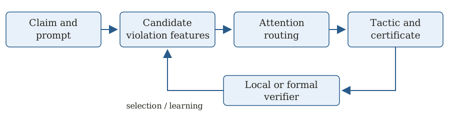
Figure 3. A proposed, not established, causal story. Search and checking costs affect which attempts succeed; learned representations may identify violations; attention can route a candidate; and learning from accepted outputs may reinforce the successful route. Testing these causal links requires interventions, not attention maps or verbal traces alone.
H1: search and checking costs.
If models choose the more promising route, counterexample attempts should increase when witnesses are easier to find (larger ), proofs cost more (larger ), or witnesses are cheaper to check. For sparse violations, the local iid model in Proposition 8.2 predicts initial success approximately , because the binomial expansion gives for fixed . Under externally uniform proposals, ; for free model search it must be estimated from the model’s prompt-dependent candidate distribution. The iid law is a search baseline, not causal evidence for H1. The adaptive hazard product (Proposition 8.3) is an identity, not a competing explanation; testing feedback requires randomized feedback and held-out predictions from independently specified or fitted hazards. An asymptotic construction may require substantial proof. A short symbolic proof can also be cheaper than finding a rare witness. Under a pure cost explanation, no counterexample preference should remain after model-specific utilities are matched.
H2: capacity hypothesis for learned max-violation routing.
An open-weight model may encode candidate-level violation scores in its residual stream, route the largest score through one or more attention heads, and increase the -token logit through downstream MLPs. From Proposition 8.4, adding distractors imposes an approximately margin requirement for a unique witness. The causal signature is not simply whether a probe can read that information. Choosing a route, constructing a witness, and checking its validity are different jobs. A selector intervention changes choice log-odds; a constructor intervention changes verified-witness rate when the route is forced; a checker intervention changes error detection. One effect need not imply another. Compare each targeted intervention with random patches and controls for general capability loss.
H3: verifier-gated amplification.
Outcome filtering, reinforcement learning from verifiable rewards, rejection sampling, or expert iteration can all enrich a tactic that yields accepted certificates more often. Under the fixed-rate idealization, Proposition 8.7 predicts linear log-odds across rounds. A controlled training experiment should therefore manipulate the two acceptance rates while holding the raw tactic frequency fixed. Process-supervision methods reward valid intermediate progress [39, 40]; we hypothesize that this can weaken a short-certificate advantage.
9.1 Alternatives that can mimic the same output
Corpus and retrieval priors.
Training text may contain stereotyped phrases such as “consider the case ” or memorized counterexamples. A model can retrieve such a pattern without search. Novel symbols, semantic-preserving renamings, contamination checks, and paired paraphrases test this explanation.
Instruction following and mathematical sycophancy.
“Prove that” prompts can suppress falsification even when the statement is false, as false-theorem evaluations demonstrate [2, 3]. Conversely, “find a flaw” prompts inflate counterexample attempts. The semantic-dual control and a full prompt-factorial are therefore indispensable.
Tool affordances.
Code, SMT solvers, finite enumerators, and proof assistants change the action space. A counterexample rate that rises only when brute-force execution is available is scaffold preference, not necessarily a property of the base model. Formal proof tools can also narrow or remove the verification asymmetry by checking both proofs and disproofs; they do not equalize search or certificate cost [41, 11].
Observation and publication selection.
Initial routing, strategy switching, mathematical validity, and reporting are four separate filters. Proposition 8.6 gives their exact odds decomposition and retains invalid-but-reported artifacts rather than assuming them away. A surprising terminal counterexample can therefore dominate the public record even when initial counterexample routing is no more common than proof routing. A celebrated result can establish mathematics without estimating any population tactic rate.
Finally, a model’s written reasoning need not reveal its internal computation: it can be post-hoc or respond to irrelevant prompt details [27]. Use open models and predeclared interventions; check robustness because activation-patching choices can change localization conclusions [42]. Arithmetic studies offer a methodological precedent [43], but no published result known to us establishes a proof-versus-counterexample circuit.
10. Testing the Competing Explanations
Main idea.
To measure preference, offer a proof task and a counterexample task that are equally promising for the model, then observe its choice. To explain that choice, change one possible cause—cost, wording, tools, training, or internal components—while controlling the others. Record failures and strategy switches, not just successful final answers. This section proposes those experiments; none was conducted for this survey.
10.1 Benchmark construction
Tier A: exactly controlled finite claims.
Generate predicates over finite sets or Boolean assignments with known domain size , violation count , and hence witness density . Factorial construction independently varies , reference-certificate length (or the shortest certificate within a finite enumerated proof grammar), surface length, and topic vocabulary. Enumerate the full domain to establish truth and to validate every proposed witness. Create true and false twins by changing one constant, quantifier, or hypothesis while preserving token-level similarity. Include claims with rare witnesses and short algebraic proofs, because they reverse the naive “counterexamples are easy” ordering. The raw ratio predicts hit rates only when candidate selection is externally forced to be uniform. In free model search, estimate the model’s effective witness mass from held-out candidate samples.
Tier B: natural and formal mathematics.
Sample universal statements from Lean’s mathlib and other licensed formal corpora. Retain the verified original as a true item; create a false twin by minimally deleting a hypothesis or perturbing a bound, following the general mutation strategy used in counterexample work [44]. Require a kernel-checked proof for every true item and a kernel-checked or executable witness for every false item. Experts audit the mapping between natural language and the formal statement; Lean checking alone does not guarantee translation faithfulness. Cover algebra, number theory, combinatorics, analysis, and finite structures, and reserve temporally new problems for contamination-resistant evaluation.
The matched portfolio.
For each topic and difficulty band, pair one true claim with an available proof and one false claim with an available counterexample. Calibrate generation and verification cost in a pilot using independent solvers. In a separate split, force each model down both tactics to estimate model-specific verified utility, then pair within a preregistered caliper and use item cross-over and fixed effects. Tell the model which portfolio claim is verified true and which is verified false, so truth inference is not the choice being measured. Create four objective-cost cells: short–short, short–long, long–short, and long–long for . The crossed cells estimate sensitivity to objective certificate economics. Only the held-out, model-specific utility-matched subset is used to estimate ; without that calibration, all cells measure task-selection bias rather than revealed preference.
10.2 Protocol and interventions
Use exact, dated model identifiers and freeze all provider settings. Include closed frontier systems for behavior and open-weight reasoning models for behavior plus internals. For each item and seed:
-
Present a neutral prompt and allow an unconstrained response. Code the initial route, checkpoint occupancies, switches, and terminal artifact with a preregistered, human-validated scheme. Do not elicit a truth probability in the same run, because elicitation can change the subsequent policy.
-
On a paired replica, require one first label from , then allow completion under the same token/tool budget. Record branch changes, tool calls, tokens, and wall-clock time. The natural-versus-labeled contrast estimates measurement reactivity.
-
Verify the final artifact with Lean, an SMT solver, or the executable predicate. Expert review audits semantics but never substitutes an LLM judge for mathematical validity.
-
On a separate replica, elicit truth confidence for calibration and compare it with tactic choice.
Cross the following interventions while matching total compute:
Table 4. Interventions that separate proposed mechanisms from confounds.
| Factor | Levels | Diagnostic contrast |
|---|---|---|
| Framing | prove; disprove; prove or disprove; neutral | Instruction prior and sycophancy |
| Semantic dual | disprove a universal; prove its existential negation | Lexical framing with identical certificate |
| Witness mass | uniform sweep; sampled model proposals | Raw versus effective iid search mass; adaptive survival hazards under feedback |
| Certificate cost | crossed short/long proof and witness | Revealed cost sensitivity and matched intercept |
| Affordance | no tool; code; SMT; Lean; verifier feedback | Base policy versus scaffold effect |
| Budget | tokens, calls, and parallel samples varied separately | Search scaling and strategy-switch hazards |
10.3 Metrics and preregistered analysis
Primary outcomes are in model-specific utility-matched portfolios, initial-route , terminal-route , verified proof rate, invalid-witness rate, false-proof rate, and verified success per tokens or tool calls. Secondary outcomes are route occupancy, the full initial-to-terminal switching matrix, adaptive hit hazards, time to the first valid certificate, Brier score for truth belief, and robustness across templates and domains. Report initial allocation, terminal artifact, and success separately; collapsing them is a category error.
Fit Equation (6) with model, item, and template effects. Estimate item-clustered intervals, correct multiplicity for secondary contrasts, and publish a prospective power analysis for the utility-matched intercept. Use a model-family cluster bootstrap only if the study includes enough independently trained families to support population inference; otherwise report exact snapshots descriptively. Randomize pair order, tactic-token labels, notation, and surface length. Release all invalid outputs and verifier logs so that selective examples cannot drive the conclusion.
10.4 Training and mechanistic causal tests
Starting from the same open base model, run a balanced factorial that varies: (i) proof versus counterexample frequency in supervised data; (ii) outcome-only versus process reward; (iii) per-tactic verifier acceptance; and (iv) certificate length. Match examples, updates, tokens, optimizer, and random seeds. The amplification account predicts approximately linear tactic log-odds across filtering rounds when acceptance rates are stationary (Equation (26)); a frequency-only account instead tracks the raw curriculum even when acceptance is held fixed.
For internal-component tests, use probes only to nominate components, then alter their activations between semantic-dual and true/false twins, remove candidate-to-output paths, or steer the hypothesized direction. Measure choosing, constructing, and checking separately. A selector changes under natural or constrained choice; it need not change validity conditional on the chosen tactic. A witness constructor changes at matched compute. A checker changes detection, rejection, or calibration of invalid candidates. Each effect must generalize across templates and domains and spare matched proof retrieval and generic language performance. Random components, equal-norm noise, and capability-matched paths are negative controls.
10.5 Predictions that risk the position
Table 5 pairs each hypothesis with an observation that would count against it. These are proposed tests, not results of this survey.
Table 5. Preregistered predictions and observations that would count against the proposed explanation.
| Hypothesis | Predicted signature | Disconfirming pattern |
|---|---|---|
| Certificate economics | Allocation changes with independently varied search opportunity and cost. Test feedback by randomization and held-out success predictions from independently specified or fitted hazards | No preregistered relation under independent mass/cost interventions with adequate power |
| Witness-routing hypothesis | Distractors require an approximately margin; a targeted intervention changes the relevant selector or constructor estimand | No decodable violation signal or no selective causal effect |
| Verifier amplification | Log-odds drift linearly with filtering round and acceptance-rate gap | Drift follows data frequency after acceptance is matched |
| Stable residual policy bias | Positive utility-matched is stable across order, labels, paraphrases, tools, and budgets; the separate dual-frame gap is small | The preregistered pattern is absent across independent controls with adequate power |
11. Objections, Boundary Conditions, and Implications
“A disproof is itself a proof.”
Correct. Formally, refuting means proving . Our distinction is between a witness-producing existential certificate and a derivation that establishes a universal claim. It applies most cleanly to with cheaply decidable . It need not apply to mixed quantifiers, nonconstructive negations, or statements whose counterexamples require long admissibility proofs. In particular, refuting an asymptotic claim requires a construction and argument that work for arbitrary ; one bad finite instance for fixed parameters is not enough.
“Proofs can compress the whole domain.”
Yes, and this is the main limitation of Proposition 8.2. An induction, invariant, or algebraic identity can certify a universal statement without enumeration. Proof complexity makes the relevant cost depend on the proof system: Cook and Reckhow give the general framework, while Haken proves an exponential resolution lower bound for pigeonhole-principle tautologies [45, 46]. Other claims have one-line proofs and extremely sparse counterexamples. The paper predicts cost-sensitive allocation, not a universal complexity ordering.
“Frontier internals are inaccessible.”
Behavioral conclusions can be drawn from closed models if versions and interfaces are fixed, but mechanistic conclusions cannot be transferred merely because an open model has similar benchmark accuracy. We therefore separate frontier behavioral measurement, open-weight causal analysis, and small-model training causality. Agreement across these levels strengthens an explanation; disagreement is itself a result.
The word “intrinsic” also needs a level. It can mean that an architecture logically forces a sign, that a symmetric training procedure systematically induces a sign, or that one trained model has a stable residual policy bias. Proposition 8.5 rules out only the first. Repeated symmetric training runs with tactic-label swaps test the second; utility-matched can support only the third.
“Reasoning traces show the strategy directly.”
Not necessarily. Chain-of-thought can omit, rationalize, or misstate causal features [27]. We compare unconstrained responses with a constrained tactic-label condition and report the gap as measurement reactivity. Mechanistic claims additionally require causal activation interventions.
11.1 What would change our view
We would reject a stable residual policy preference if utility-matched is null or negative with adequate power; if a positive raw is mostly invalid witnesses; or if a preregistered pattern across framing, tools, and label-reactivity controls accounts for the effect. Semantic duals contribute a separate lexical-frame gap rather than an . We would strengthen the claim from “conditional gravity” toward a learned, model-level preference only if a positive utility-matched intercept generalizes across truth-balanced domains, paraphrases, budgets, and model versions, and if controlled training and causal interventions identify a tactic-specific mechanism beyond corpus frequency. Even then, Proposition 8.5 rules out calling the sign an architectural necessity.
11.2 Implications for training and evaluation
First, prove-or-disprove benchmarks should score four quantities separately: strategy choice, certificate validity, efficiency, and truth calibration. Second, curricula should balance proofs, disproofs, and abstentions while varying certificate length and effective witness mass; otherwise verifier filtering can silently collapse tactic diversity. Third, process supervision should reward reusable proof progress and admissibility checks, not only short terminal witnesses. Fourth, systems deployed for mathematical research should preserve the constructive value of counterexample search while escalating every candidate to an independent checker. A model willing to challenge a consensus can be scientifically valuable; a model willing to assert an invalid witness or fabricate a proof is not.
The broader lesson is methodological. “Preference” should name a measured policy contrast under controlled opportunity, not an anthropomorphic gloss on a few memorable outputs. Certificate economics explains why falsification can be attractive, Transformer attention has the capacity to route a salient witness, and validity and reporting filters can amplify terminal behavior. Initial allocation, intermediate occupancy, and the published endpoint can differ. Only experiments can determine whether those mechanisms are active in a given frontier system.
12. Conclusion
Frontier models now contribute to mathematical research through several distinct channels: benchmark solving, new constructions, human-guided proofs, research disproofs, and formalization. The strongest evidence comes from inspectable artifacts paired with a precise record of the system, task, interaction, and verification. Headline success alone leaves most of that record unspecified.
Our bounded cohorts do not establish a general preference for falsification. The fixed FrontierMath Erdős run produced one proof and one disproof; across the fixed and nonuniform further search, three statements were resolved affirmatively and two negatively. Selected announcements and construction-oriented registries answer different questions. Counting every example as a counterexample, or every published disproof as an initially chosen tactic, would manufacture the conclusion the survey is meant to test.
The theory explains why counterexample search can nevertheless be attractive. Effective witness mass, certificate cost, informative feedback, and downstream selection can favor it in a particular environment. None is an unconditional theorem about mathematical difficulty or Transformer psychology. The finite oracle asymmetry assumes an unstructured domain; an asymptotic disproof may need an infinite construction family and a substantial derivation. Softmax routing establishes representational capacity, not a discovered mechanism. Utility-shift and reporting-selection results explain why observed outcomes alone cannot identify an intrinsic preference.
The position is therefore methodological as well as explanatory: study the whole research process, keep outcome, certificate, and workflow separate, and measure initial allocation independently from switching and final acceptance. Future evaluations should match utilities, include semantic-dual controls, retain failed attempts, and verify the intended statement. Such measurements could support a learned tendency to falsify, reveal a context-dependent advantage, or reject the premise. Each would be more informative than treating a compelling collection of discoveries as an already established law.
Disclosure of AI Assistance
This work was prepared with extensive assistance from GPT-6 Astra Ultra. The model assisted with literature search and synthesis, evidence extraction and organization, mathematical formulation and proof drafting, manuscript drafting and revision, and LaTeX, tables, figures, and reproducibility scripts. AI-assisted checking and separate agent reviews were also used; these do not constitute independent human peer review or replace expert verification of sources, mathematics, and interpretations. The reported survey statistics are derived from published sources. Responsibility for the final content, claims, citations, and any errors remains with the human authors.
References
- T. Gowers. What sort of maths are LLMs good at? 2026. First-hand mathematical discussion, 12 August 2026. https://gowers.wordpress.com/2026/08/12/what-sort-of-maths-are-llms-good-at/.
- I. Petrov, J. Dekoninck, and M. Vechev. BrokenMath: A benchmark for sycophancy in theorem proving with LLMs. Proceedings of the 43rd international conference on machine learning, PMLR, 306, 2026. https://arxiv.org/abs/2510.04721.
- J. Dekoninck, T. Gehrunger, K. Rögnvaldsson, C. Sun, and M. Vechev. BrokenArXiv: How often do LLMs claim to prove false theorems? MathArena research report, 2026. Accessed 2026-08-19. https://matharena.ai/brokenarxiv/.
- Y. Li, J. Kuang, H. Huang, Z. Xu, X. Liang, Y. Yu, W. Lu, Y. Li, X. Tan, C. Qu, Y. Shen, H.-T. Zheng, and P. S. Yu. One example shown, many concepts known! Counterexample-driven conceptual reasoning in mathematical LLMs. Proceedings of the 42nd international conference on machine learning, PMLR, 267, pp. 35168–35185, 2025. https://proceedings.mlr.press/v267/li25ax.html.
- S. Sinha, S. Goel, P. Kumaraguru, J. Geiping, M. Bethge, and A. Prabhu. Can language models falsify? Evaluating algorithmic reasoning with counterexample creation. Second conference on language modeling, 2025. https://openreview.net/forum?id=M7cl4Ldw61.
- I. Tzachristas, G. Tzachristas, and A. Sui. Open problems solved by LLMs? A survey of verifiable mathematical discovery. Proceedings of the big picture v2: Crafting a research narrative, Association for Computational Linguistics, pp. 10–21, 2026. https://aclanthology.org/2026.bigpicture-main.2/.
- S. R. Raiyan, M. Kabir, H. Mahmud, M. K. Hasan, and S. Ananiadou. Artificial intelligence for mathematical reasoning: An integrated survey of language models, neuro-symbolic systems, and verified discovery. 2026. arXiv:2606.08728v4, 26 July 2026. https://arxiv.org/abs/2606.08728v4.
- A. Novikov, N. Vũ, M. Eisenberger, E. Dupont, P.-S. Huang, A. Z. Wagner, S. Shirobokov, B. Kozlovskii, F. J. R. Ruiz, A. Mehrabian, M. P. Kumar, A. See, S. Chaudhuri, G. Holland, A. Davies, S. Nowozin, P. Kohli, and M. Balog. AlphaEvolve: A coding agent for scientific and algorithmic discovery. Google DeepMind, 2025. White paper. https://storage.googleapis.com/deepmind-media/DeepMind.com/Blog/alphaevolve-a-gemini-powered-coding-agent-for-designing-advanced-algorithms/AlphaEvolve.pdf.
- T. Luong and E. Lockhart. Advanced version of Gemini with Deep Think officially achieves gold-medal standard at the international mathematical olympiad. Google DeepMind research report, 2025. Published 21 July 2025; accessed 19 September 2026. https://deepmind.google/blog/advanced-version-of-gemini-with-deep-think-officially-achieves-gold-medal-standard-at-the-international-mathematical-olympiad/.
- B. Georgiev, J. Gómez-Serrano, T. Tao, and A. Z. Wagner. Mathematical exploration and discovery at scale. 2025. Version 3, 22 December 2025. https://arxiv.org/abs/2511.02864.
- T. Hubert and others. Olympiad-level formal mathematical reasoning with reinforcement learning. Nature, 651, pp. 607–613, 2026. https://doi.org/10.1038/s41586-025-09833-y.
- T. Feng, T. Trinh, G. Bingham, J. Kang, S. Zhang, S. Kim, K. Barreto, C. Schildkraut, J. Jung, J. Seo, C. Pagano, Y. Chervonyi, D. Hwang, and others. Semi-autonomous mathematics discovery with Gemini: A case study on the Erdős problems. 2026. Version 3, 5 February 2026. https://arxiv.org/abs/2601.22401.
- T. Feng, T. H. Trinh, G. Bingham, D. Hwang, Y. Chervonyi, J. Jung, J. Lee, C. Pagano, S. Kim, F. Pasqualotto, S. Gukov, and others. Towards autonomous mathematics research. 2026. Version 3, 6 March 2026. https://arxiv.org/abs/2602.10177.
- M. Firsching, P. Lezeau, S. Mercuri, M. Z. Horváth, Y. Dillies, C. Sönne, E. Wieser, F. Zhang, T. Hubert, B. Agüera y Arcas, and P. Kohli. Formal conjectures: An open and evolving benchmark for verified discovery in mathematics. 2026. https://arxiv.org/abs/2605.13171.
- N. Alon, T. F. Bloom, W. T. Gowers, D. Litt, W. Sawin, A. Shankar, J. Tsimerman, V. Wang, and M. M. Wood. Remarks on the disproof of the unit distance conjecture. 2026. https://arxiv.org/abs/2605.20695.
- Epoch AI. FrontierMath Tier 4 (v2). Benchmark documentation, 2026. Released 12 June 2026; accessed 19 September 2026. https://epoch.ai/benchmarks/frontiermath-tier-4-v2.
- M. Abouzaid, N. Srivastava, R. Ward, and L. Williams. First proof second batch. 2026. Report dated 10 June 2026; submitted 16 June 2026. https://arxiv.org/abs/2606.18119.
- Anonymous. A counterexample to the Jacobian Conjecture. Mathematical manuscript hosted by Ulam AI, 2026. Dated 20 July 2026; verifies the example announced by Levent Alpöge and credits Fable for the work leading to it; no named author is given. https://www.ulam.ai/research/jacobian.pdf.
- OpenAI. Ten advances in mathematics and theoretical computer science. Research publication, 2026. Published 1 August 2026; manuscript updated 6 August 2026; Lean certificates at https://github.com/openai/ten-proofs. https://openai.com/index/ten-advances-in-mathematics/.
- T. Adamczewski and G. Burnham. Announcing FrontierMath Erdős. Epoch AI benchmark report, 2026. Published 1 September 2026; paper at https://epoch.ai/files/frontiermath-erdos.pdf. https://epoch.ai/latest/announcing-frontiermath-erdos.
- Anthropic. Formalizing fermat’s last theorem. Research report and formal artifact, 2026. Published 4 September 2026; Lean source at https://github.com/anthropics/fermats-last-theorem. https://www.anthropic.com/research/formalizing-fermats-last-theorem.
- OpenAI. On the Navier–Stokes millennium prize problem. Research publication, 2026. Published 8 September 2026; updated 10 September 2026; Lean artifact at https://github.com/openai/NavierStokesAndEuler. https://openai.com/index/navier-stokes-solution/.
- E. Y. Wang, S. R. Motwani, J. V. Roggeveen, E. Hodges, D. Jayalath, C. London, K. Ramakrishnan, J. Foerster, C. Zhang, F. Cipcigan, P. Torr, and A. Abate. Measuring progress in reasoning toward mathematical discovery with automatic verification. 2026. Version 2, 10 September 2026; ICML AI4Math Best Paper Award. https://arxiv.org/abs/2603.15617.
- Epoch AI. FrontierMath: Open problems. Evolving benchmark and results ledger, 2026. Snapshot accessed 19 September 2026; last policy update 16 September 2026. https://epoch.ai/frontiermath/open-problems.
- OpenAI. An OpenAI model has disproved a central conjecture in discrete geometry. Research report, 2026. Accessed 2026-08-19. https://openai.com/index/model-disproves-discrete-geometry-conjecture/.
- Anthropic. Discovering cryptographic weaknesses with Claude. Research report, 2026. Published 28 July 2026; contains Anthropic’s retrospective attribution of the Jacobian-conjecture counterexample to Claude Fable 5. https://www.anthropic.com/research/discovering-cryptographic-weaknesses.
- M. Turpin, J. Michael, E. Perez, and S. R. Bowman. Language models don’t always say what they think: Unfaithful explanations in chain-of-thought prompting. Advances in neural information processing systems, 36, 2023. https://proceedings.neurips.cc/paper_files/paper/2023/hash/ed3fea9033a80fea1376299fa7863f4a-Abstract-Conference.html.
- U. Jang and E. K. Ryu. Point convergence of nesterov’s accelerated gradient method: An AI-assisted proof. 2026. arXiv:2510.23513v2, 19 January 2026; originally posted October 2025. https://arxiv.org/abs/2510.23513v2.
- K. Cobbe, V. Kosaraju, M. Bavarian, M. Chen, H. Jun, L. Kaiser, M. Plappert, J. Tworek, J. Hilton, R. Nakano, C. Hesse, and J. Schulman. Training verifiers to solve math word problems. 2021. https://arxiv.org/abs/2110.14168.
- C. Snell, J. Lee, K. Xu, and A. Kumar. Scaling LLM test-time compute optimally can be more effective than scaling parameters for reasoning. International conference on learning representations, 2025. https://proceedings.iclr.cc/paper_files/paper/2025/hash/1b623663fd9b874366f3ce019fdfdd44-Abstract-Conference.html.
- A. Setlur, N. Rajaraman, S. Levine, and A. Kumar. Scaling test-time compute without verification or RL is suboptimal. Proceedings of the 42nd international conference on machine learning, PMLR, 267, pp. 54058–54094, 2025. https://proceedings.mlr.press/v267/setlur25a.html.
- S. Bubeck, C. Coester, R. Eldan, T. Gowers, Y. T. Lee, A. Lupsasca, M. Sawhney, R. Scherrer, M. Sellke, B. K. Spears, D. Unutmaz, K. Weil, S. Yin, and N. Zhivotovskiy. Early science acceleration experiments with GPT-5. 2025. arXiv:2511.16072. https://arxiv.org/abs/2511.16072.
- OpenAI. Ten advances in mathematics and theoretical computer science. OpenAI, 2026. Manuscript updated 6 August 2026; ten numbered entries in the abstract. https://cdn.openai.com/pdf/ten-proofs-oai.pdf.
- T. Adamczewski and T. F. Bloom. FrontierMath Erdős. Epoch AI, 2026. Companion benchmark paper; Sections 3.2, 4.1–4.2 and Appendix B. https://epoch.ai/files/frontiermath-erdos.pdf.
- Epoch AI. The core in approval-based committee elections. 2026. FrontierMath Open Problems solution update; snapshot 19 September 2026. https://epoch.ai/frontiermath/open-problems/committee-election.
- Epoch AI. A presentation of the absolute galois group of . 2026. FrontierMath Open Problems solution update and verification caveat; snapshot 19 September 2026. https://epoch.ai/frontiermath/open-problems/q2-absolute-galois.
- MathArena. Competitions and BrokenArXiv monthly dataset inventory. 2026. Literature cutoff 19 September 2026; mutable monthly inventory, independently rechecked 20 September 2026. https://matharena.ai/competitions.
- A. Vaswani, N. Shazeer, N. Parmar, J. Uszkoreit, L. Jones, A. N. Gomez, L. Kaiser, and I. Polosukhin. Attention is all you need. Advances in neural information processing systems, 30, pp. 5998–6008, 2017. https://proceedings.neurips.cc/paper/2017/hash/3f5ee243547dee91fbd053c1c4a845aa-Abstract.html.
- H. Lightman, V. Kosaraju, Y. Burda, H. Edwards, B. Baker, T. Lee, J. Leike, J. Schulman, I. Sutskever, and K. Cobbe. Let’s verify step by step. International conference on learning representations, 2024. https://openreview.net/forum?id=v8L0pN6EOi.
- J. Uesato, N. Kushman, R. Kumar, F. Song, N. Siegel, L. Wang, A. Creswell, G. Irving, and I. Higgins. Solving math word problems with process- and outcome-based feedback. 2022. https://arxiv.org/abs/2211.14275.
- K. Yang, A. M. Swope, A. Gu, R. Chalamala, P. Song, S. Yu, S. Godil, R. J. Prenger, and A. Anandkumar. LeanDojo: Theorem proving with retrieval-augmented language models. Advances in neural information processing systems, 36, 2023. https://proceedings.neurips.cc/paper_files/paper/2023/hash/4441469427094f8873d0fecb0c4e1cee-Abstract-Datasets_and_Benchmarks.html.
- F. Zhang and N. Nanda. Towards best practices of activation patching in language models: Metrics and methods. International conference on learning representations, 2024. https://openreview.net/forum?id=Hf17y6u9BC.
- A. Stolfo, Y. Belinkov, and M. Sachan. A mechanistic interpretation of arithmetic reasoning in language models using causal mediation analysis. Proceedings of the 2023 conference on empirical methods in natural language processing, pp. 7035–7052, 2023. https://doi.org/10.18653/v1/2023.emnlp-main.435.
- Z. Li, Z. Li, K. Yang, X. Ma, and Z. Su. Learning to disprove: Formal counterexample generation with large language models. 2026. Withdrawn ICLR 2026 submission. https://arxiv.org/abs/2603.19514.
- S. A. Cook and R. A. Reckhow. The relative efficiency of propositional proof systems. Journal of Symbolic Logic, 44, no. 1, pp. 36–50, 1979. https://doi.org/10.2307/2273702.
- A. Haken. The intractability of resolution. Theoretical Computer Science, 39, no. 2–3, pp. 297–308, 1985. https://doi.org/10.1016/0304-3975(85)90144-6.
Appendix A. Complete Derivations
This appendix supplies every algebraic and probabilistic step omitted from the main exposition.
Read the main-text explanations first: the purpose here is to check their mathematical steps, not to introduce the argument. Correct algebra establishes what follows from stated assumptions; it is not empirical validation of those assumptions or evidence that frontier models implement these mechanisms.
Reading map.
Appendix A.1 balances finding a certificate against producing it without errors: a shorter answer need not be easier to discover. Appendix A.2 shows how attention can route an already recognized witness, not how that witness is recognized or constructed. Appendix A.3 explains why reported final answers can hide initial strategy choice. Appendix A.4 shows how filtering for success can amplify either proofs or counterexamples, whichever has the assumed acceptance advantage. Appendix A.5 computes the expected search time when a finite domain is inspected in random order without repeating candidates.
A.1 Accepted-answer odds under fallible generation
Corollary A.1 (Accepted-answer odds). Let be the terminal tactic in a one-branch attempt with no strategy switch, and let and denote the events that the task is false and true. Assume and , and assume
Conditional on and , counterexample search makes an integer number of independent proposals from a fixed distribution , and the counterexample set has effective mass . Conditional on and , proof search finds a viable proof plan or skeleton with probability . A counterexample and a proof certificate contain indispensable generated decisions, respectively. Within each selected tactic, these decisions are conditionally independent with common correctness probability and independent of truth and search outcomes. The verifier rejects if the selected tactic is incompatible with the task’s truth value or if search fails. Conditional on compatible truth and successful search, it accepts if and only if all indispensable decisions are correct, with no additional failure mode. Define
where denotes verifier acceptance. Then
and exactly when Equation (19) holds.
Proof. Let be the event that at least one of the proposals hits a counterexample, and let be the event that all indispensable counterexample-certificate decisions are correct. The assumptions give
The middle equality follows from the effective-mass calculation in Proposition 8.2. For the last equality, independence of the decisions makes the probability that all are correct equal to
By assumption, conditional on , the acceptance event is exactly . The conditional chain rule gives
Similarly, let be the event that proof search finds a viable proof plan or skeleton, and let be the event that all indispensable proof-certificate decisions are correct. Then
By assumption, conditional on , the acceptance event is exactly . Applying the conditional chain rule step by step gives
All displayed factors are strictly positive. We may therefore divide without changing the direction of an inequality and take the strictly increasing natural logarithm:
Because
moving the first logarithm to the other side gives
which is exactly Equation (19). Reversing these equivalences proves the “if” direction as well as the “only if” direction. ◻
If tactic costs , accepted answers per unit cost are . All success probabilities and costs are positive, so division and the increasing logarithm preserve the strict inequalities:
The penultimate step uses ; the last uses for .
A.2 Softmax witness-routing capacity bound
Proof of Proposition 8.4. Define the counterexample and noncounterexample partition sums
For every , the score assumption gives . Summing such terms gives
For every , it gives . There are such terms, hence
The lower bound on is positive, so
The total attention mass on is
where the final inequality follows because is decreasing for . This proves Equation (20).
Now suppose the witness is unique and for every . Define
Each exponent is at most , so
Divide the numerator and denominator of by . This yields
For the attention output,
The triangle inequality, , and another triangle inequality give
The function is increasing for , because its derivative is . Substituting the upper bound on gives
Finally, the denominator is at least one, so dropping it only enlarges the right-hand side. Therefore
Both inequalities in Equation (21) are proved. ◻
A.3 Validity, reporting, and strategy switching
Proof of Proposition 8.6. For , abbreviate
The assumed positive prior and reported cells imply and , hence . The law of total probability gives
where terms with zero may be omitted. In particular, , so Bayes’ rule applies. For each ,
Taking the ratio of the and equalities cancels the common, positive denominator:
We next expand each reporting probability without assuming validity. The events and form a disjoint partition, so the conditional chain rule gives
If one validity stratum has conditional probability zero, its joint term is zero; the stipulated arbitrary value of the corresponding is therefore multiplied by zero and cannot change the equality.
Finally, the initial-route events form a finite partition. A second application of the law of total probability yields
Substituting this expression for and the preceding expression for into Equation (28) gives Equation (23) exactly. Notice that no equality between and was used; all switches are retained in .
Suppose now that reporting implies validity, so up to a null event. Then, for each terminal route ,
Consequently , including the cases where the invalid stratum itself has probability zero, and
Substitution into Equation (28), followed by splitting the positive ratio , gives
which is Equation (24).
For the conditional claim, fix an such that, for each , both and . Replace every probability in the preceding argument by . Bayes’ rule and both conditional chain-rule steps remain valid under this conditional probability measure. Moreover,
so the first odds factor becomes , while the validity and reporting factors acquire the same conditioning on . This proves the final assertion and completes the proof. ◻
Explicit nonidentification example.
Let take only the two routes, set , and consider these three valid parameter settings:
For settings 1, 2, and 3, respectively, the three odds factors in Equation (24) are
Each factor changes between at least two settings, yet all yield the same reported route distribution. Indeed, the two joint reported probabilities are in every setting: the relevant products are
Thus and for both routes in all three settings. Even knowing overall reporting prevalence would not distinguish them. Separately, let , let , and set both rows of to . Then, for either terminal route,
Keeping validity and reporting fixed therefore yields identical observed outputs for every , although the initial odds vary. Terminal output counts cannot resolve initial strategy allocation without further information about switching.
A.4 Verifier-induced mode amplification
Proof of Proposition 8.7. Let denote the terminal tactic and let denote acceptance. At round , the model and filter assumptions are
The law of total probability gives
This quantity is positive because and both success rates are positive. Bayes’ rule therefore gives
By assumption, the next unconstrained Bernoulli marginal fit sets its mode parameter to the accepted-population frequency, so . This proves Equation (25).
Subtracting the recurrence from one and putting terms over the same denominator gives
Both and are positive. Dividing their expressions cancels the shared denominator:
We now prove by induction that
For , the exponent is zero and the right-hand side equals . Assume Equation (29) holds for . The one-step odds recurrence then gives
Thus the formula holds for every nonnegative integer .
Taking logarithms of positive quantities and using yields
which is Equation (26). If , the odds in Equation (29) tend to infinity, forcing . If the ratio is less than one, the odds tend to zero, forcing . If it equals one, the odds and hence remain equal to their initial values. ◻
A.5 Search without replacement
The main text gives both the iid specialization and an adaptive hazard law. Exact finite enumeration without replacement has a related closed form.
Lemma A.2 (First violation in a random ordering). Let and be integers with , and suppose exactly of the points violate a universal claim. Inspect all points in a uniformly random order, and let be the position of the first violation. Then
Proof. For , the event means that none of the first positions contains a violation. Equivalently, all violating points lie among the remaining positions. Of the equally likely sets of violation positions, exactly satisfy this condition. Therefore
For , the probability is zero because fewer than positions remain. We derive the needed tail sum directly. For every realized value , exactly the indicators with equal one, so
The sum is finite; taking expectations term by term and using yields
It remains to derive the binomial sum. Pascal’s identity gives, for ,
For , putting the two terms on the equivalent left-hand side over a common denominator gives
At the endpoint , the same identity reads , using . Summing the difference from to telescopes:
Substituting and the two derived identities now gives
Expanding the factorials completes the simplification:
◻
Appendix B. Minimal Reproducible Evaluation Protocol
For each released result, report: model identifier and access date; system and user prompts; decoding parameters; context and output limits; tool versions; parallel sample count; truth label and proof system; verifier source and logs; whether a route label was elicited or forced; the complete visible response; initial, checkpoint, and terminal route annotations; strategy switches; certificate length; verification cost; final validity; reporting status; and all exclusion rules. Cluster the train, validation, and test split by source theorem before mutation so that true/false twins never cross splits.
The primary neutral behavioral prompt should avoid both asserting truth and forcing a route declaration:
Determine the status of the following claim and give a certificate that can be checked under the stated formal system. A counterexample must satisfy every hypothesis and violate the conclusion; a proof must justify every inference.
On a randomized paired replica, the optional labeled arm inserts the following sentence before the request for a certificate:
Before solving, output exactly one provisional route label from
[COUNTEREXAMPLE],[PROOF],[MIXED], or[ABSTAIN].
The label is provisional: subsequent switches and the terminal artifact are recorded separately. The natural-versus-labeled contrast estimates measurement reactivity and must not be pooled as if the two prompts sampled the same policy. The portfolio prompt should hide tactic names behind randomized labels until after choice, preventing token semantics from contaminating . Analysis code must decode those labels only after model responses are frozen.
Appendix C. Evidence Coding and Reproduction
The supplement contains extraction records, not a synthetic dataset of unobserved model trials. Its unit of analysis depends on the file. cohorts.csv holds bounded cohort definitions and aggregate counts; discoveries.csv holds individually classified reported outcomes; preserves original metric names, units, prompt conditions, and precision. supports the timeline, while supports the workflow table. The codebook, search log, classification audit, and review notes are separate files so that a reader can inspect judgments as well as numbers.
C.1 A reproducible decision sequence
The following sequence is our coding rule, not a model experiment. First identify the source’s actual target. Retain the quantifiers and distinguish a named conjecture from an associated extremal record. Next identify exactly what was established and by which check. Code an affirmation only relative to that target; code a refutation only if its negation was established. If a bound improved without resolving the target, retain partial progress. When an entry contains several targets, retain that fact and document the choice of aggregation rather than silently selecting the most dramatic part.
Then classify the certificate independently. A finite witness is an explicitly specified finite object with checkable required properties. A construction family supplies objects at varying sizes and normally needs a uniform argument. An existence argument establishes an object without necessarily producing a usable instance. A general derivation proves a statement through a chain of lemmas or transformations. Mixed certificates combine these burdens. These categories refer to the delivered argument, not to whether a Lean file, a Python program, or an expert was used to check it.
Finally, classify the workflow. Record whether the source documents autonomous execution under a harness, substantive human mathematical guidance, an externally chosen search direction, or formalization of established mathematics. When autonomy is claimed only for the argument-generation phase, do not extend the claim to problem selection, manuscript preparation, or formal statement design. Missing information remains missing.
The registry’s own tags are preserved as metadata, not imposed as our outcome labels. For example, a task may be tagged “counterexample” because it asks whether a certain bad configuration exists. A proof that no such configuration exists is an affirmative mathematical result about nonexistence. Counting that result as a successful counterexample would reverse its meaning. Similarly, a large construction can establish a positive lower bound without negating any explicitly conjectured upper bound.
C.2 Version and denominator controls
Each source revision can change more than a headline number. A discovered prior construction changes novelty; a corrected proof changes validity; a changed attribution policy changes the human–AI category; and a removed problem changes the active denominator. The version fields therefore belong to the data, not merely the bibliography. The extraction retains reported precision. A value printed to one decimal place is not converted back into a unique integer count unless the source explicitly supplies that integer.
The four bounded cohorts must be read separately. A collection of selected announcements has no attempted-problem denominator. A systematic problem sweep can contain partial resolutions and rediscoveries. A fixed single-attempt run differs from nonuniform repeat search on the same targets. A live registry is a ledger of tasks and achievements, not a controlled run of one model. The two FrontierMath Erdős rows overlap intentionally: the extended row contains the fixed run. They must never be added together.
The reproduction script validates unique record identifiers, nonnegative integer count fields, aggregate arithmetic, and the reported outcome totals against the coded records where the ledger is complete. It builds figures and tables directly from these files. These checks detect transcription and aggregation errors; they cannot prove that a source is correct or that a judgment call is uniquely appropriate. The separate classification audit records such ambiguities.
C.3 Reading the cohort figure
The solution-type plot conditions on the outcomes included in each panel. Its bars are counts, not estimates of a common population parameter. An unresolved attempt is not secretly a proof attempt or a counterexample attempt: the public record may not say what route was explored. The full cohort denominator is therefore displayed alongside the resolved-entry breakdown, and the Gemini panel is labeled “addressed” because partial and literature-based results are included.
No confidence interval is attached to a selected showcase or a census of a dated registry. Such an interval would require a probability model for selection, sampling, or repeated execution. We also do not attach a binomial test against one half. Even with exact counts, unequal truth-status prevalence, certificate costs, and externally assigned routes make that null hypothesis unmotivated.
C.4 Reproduction and updating
With Python and Matplotlib installed, run python scripts/reproduce.py from the source directory. The generated table files and vector figures are included in the source archive, so compiling the paper does not require Python. Compile main.tex with Tectonic, or use a conventional PDFLaTeX, BibTeX, PDFLaTeX, PDFLaTeX sequence. The supplement’s README records the build used for this release.
A future update should create a new dated cohort rather than overwrite the September snapshot. Preserve the earlier extraction, list changed records, and regenerate the outputs. New model experiments should have a separate run ledger with one row per attempt, including failures. That extension would permit analyses the present literature-only review cannot support.
C.5 Record-level classification ledger
Table 6. Record-level direction, resolution status, and certificate codes. Source passages, verification, workflow, and sensitivity notes are in discoveries.csv. Detail-only rows do not enter the ten-entry denominator. The fixed and extended Erdős rows repeat two mathematical results.
| Record | Direction | Status | Certificate |
|---|---|---|---|
| Gemini Erdős v3 | |||
| Erdős problem 652 | proof | affirmation | general derivation |
| Erdős problem 1051 | proof | affirmation | general derivation |
| Erdős problem 654 | disproof | partial progress | construction family |
| Erdős problem 1040 | disproof | partial progress | construction family |
| Erdős problem 397 | disproof | refutation | construction family |
| Erdős problem 935 | proof | partial progress | construction family |
| Erdős problem 659 | proof | affirmation | construction family |
| Erdős problem 1089 | other resolution | affirmation | mixed |
| Erdős problem 333 | disproof | refutation | mixed |
| Erdős problem 591 | proof | affirmation | general derivation |
| Erdős problem 705 | disproof | refutation | construction family |
| Erdős problem 992 | disproof | refutation | existence argument |
| Erdős problem 1105 | proof | affirmation | general derivation |
| OpenAI selected ten | |||
| High-dimensional sphere packing | proof | affirmation | general derivation |
| Binary and spherical codes | proof | partial progress | general derivation |
| Nonsofic groups exist | disproof | refutation | construction family |
| Connes’s rigidity conjecture | disproof | refutation | construction family |
| Arithmetic circuit complexity | proof | partial progress | general derivation |
| Quantum parallel repetition | proof | affirmation | general derivation |
| Closest vector problem | proof | partial progress | general derivation |
| Ehrhart’s volume conjecture | proof | affirmation | general derivation |
| Multicolor Ramsey numbers | proof | affirmation | construction family |
| Compactness and degeneracy conjectures | disproof | refutation | construction family |
| Compactness conjecture subresult (detail only) | disproof | refutation | construction family |
| Degeneracy conjecture subresult (detail only) | disproof | refutation | construction family |
| Erdős fixed Astra | |||
| Erdős problem 74 | disproof | refutation | existence argument |
| Erdős problem 126 | proof | affirmation | general derivation |
| Erdős all Astra attempts | |||
| Erdős problem 1 | disproof | refutation | construction family |
| Erdős problem 74 | disproof | refutation | existence argument |
| Erdős problem 126 | proof | affirmation | general derivation |
| Erdős problem 548 | proof | affirmation | general derivation |
| Erdős problem 571 | proof | affirmation | construction family |
| Open registry (19 Sep.) | |||
| The Core in Approval-Based Committee Elections | proof | affirmation | general derivation |
| Many Rational Points on a Genus-2 Curve | construction | affirmation | finite witness |
| Elliptic Curves over Q of Large Rank | construction | affirmation | finite witness |
| Hadamard Matrix of Order 668 | construction | affirmation | finite witness |
| Inverse Galois problem for the Mathieu group M23 | construction | affirmation | finite witness |
| Genus-2 curve with rational torsion of prime order at least 31 | construction | affirmation | finite witness |
| Short Superpermutations over 8, 9, and 10 | construction | affirmation | finite witness |
| Presentation of the absolute Galois group of Q2 | construction | affirmation | mixed |
Citation
Please cite this work as:
Zhao, Jinze. “Mathematical Discovery with Frontier Language Models: Progress, Practice, and Counterexample Search”. jimz7-blog.pages.dev (Sep 2026).
https://jimz7-blog.pages.dev/mathematical-discovery-with-frontier-language-models/
Or use the BibTeX citation:
@article{zhao2026mathematical-discovery-with-frontier-language-models,
  title = {{Mathematical Discovery with Frontier Language Models: Progress, Practice, and Counterexample Search}},
  author = {Zhao, Jinze},
  journal = {jimz7-blog.pages.dev},
  year = {2026},
  month = {September},
  url = {https://jimz7-blog.pages.dev/mathematical-discovery-with-frontier-language-models/}
}