Domino Fit as Constrained Perfect Matching

Abstract

Domino Fit asks for a complete tiling of an obstructed grid by two fixed dominoes: a vertical piece carrying one dot above a blank, and a horizontal piece carrying a blank to the left of two dots. Every row and column must attain a prescribed dot sum. We formulate the game as binary exact cover with linear side constraints and derive an equivalent system of orientation quotas. The row clues determine every horizontal-boundary crossing count directly, while a recurrence recovers every vertical-boundary crossing count from the column clues. These invariants support an exact solver combining bitset domains, forced placements, geometric capacity checks, and minimum-domain branching. An independent exhaustive enumerator validates four implementations on 1,682 small clue cases, giving 6,728 comparisons. Experiments include the three boards solved in the accompanying play session and 72 reproducibly generated instances. All three observed boards are uniquely solved by propagation alone. We also give a fixed-width dynamic program and establish NP-completeness for the generalized game with arbitrary holes. Efficiency claims are restricted to the implementations and workload actually measured; no universal runtime optimality is asserted.

1. Problem and research scope

The Steam version of Domino Fit supports $6\times6$, $7\times7$, and $8\times8$ boards [1]. Its in-game help and the completed play session establish the rules modeled here: cover every available square, respect obstacles, and match the row and column dot totals. Only the two orientations in Section 2 are allowed. Exchanging the dotted and blank ends changes the problem and is not a legal move in this model.

The objective is feasibility. A player needs one valid tiling; a puzzle designer may additionally need to decide uniqueness or enumerate alternatives. An efficient algorithm must distinguish these tasks and separate computation time from screen reading, animation, and mouse input.

The mathematical setting is a perfect matching of the grid graph with additional orientation counts. Prior work studies reconstruction of domino tilings from counts of horizontal pieces in rows and vertical pieces in columns; for arbitrary sub-grids this reconstruction problem is strongly NP-hard [2, Theorem 4]. Exact-cover search is a natural computational framework, following the broader approach developed by Knuth [3]. This report translates Domino Fit’s asymmetric dot rules into that framework, proves a solver tailored to the resulting constraints, and supplies reproducible experiments.

The phrase most efficient needs a specified machine, implementation, workload, and stopping condition. We compare four exact implementations under the same timing protocol and recommend the best measured practical default. We do not claim that it dominates every native-code or SAT solver. The finite board sizes in the released game are also distinct from the unbounded family used in complexity analysis.

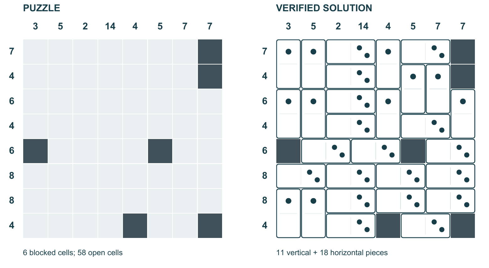
Figure 1. The actual $8\times8$ instance transcribed from the play session (left) and its independently checked unique solution (right). Dark cells are blocked. Geometry and dots are reconstructed from the recorded data, not extracted from a hidden game state.

2. An exact mathematical formulation

Number rows downward and columns rightward, starting at one. Let $B\subseteq\{1,\ldots,m\}\times\{1,\ldots,n\}$ be the blocked cells and let $\mathcal{O}$ be its complement. Set $N=|\mathcal{O}|$. The input contains nonnegative integer targets $R_i,C_j$. The legal placements are

$$V_{ij}:\ \begin{matrix}1\\0\end{matrix} \quad\hbox{on }(i,j),(i+1,j), \qquad H_{ij}:\ \begin{matrix}0&2\end{matrix} \quad\hbox{on }(i,j),(i,j+1).$$

Both cells must be open. There is an unlimited supply of each type. Introduce binary variables $v_{ij},h_{ij}$ for legal placements, defining every illegal or out-of-bounds variable to be zero. The entire game is

$$\begin{aligned} v_{ij}+v_{i-1,j}+h_{ij}+h_{i,j-1}&=1 &&((i,j)\in\mathcal{O}), && \text{(1)} \\ \sum_jv_{ij}+2\sum_jh_{ij}&=R_i &&(1\leq i\leq m), && \text{(2)} \\ \sum_iv_{ij}+2\sum_ih_{i,j-1}&=C_j &&(1\leq j\leq n), && \text{(3)} \\ v_{ij},h_{ij}&\in\{0,1\}. &&&& \text{(4)} \end{aligned}$$

There are at most $(m-1)n+m(n-1)$ variables. Each selected variable covers two cells and contributes dots exactly where the game places them. Thus Equation (1) prevents overlap and omissions, while Equation (2), Equation (3) enforce the clues. Conversely, every successful assignment satisfies these equations. Feasible binary vectors and legal tilings are therefore in bijection.

In graph language, vertices are open cells and edges join orthogonally adjacent open cells. Selected edges form a perfect matching, with dot sums as side constraints. Checkerboard coloring makes the graph bipartite, but does not eliminate those side constraints. Plain exact cover without the clue equations solves only the geometry.

The model can also be submitted to an integer or constraint-programming solver. CP-SAT accepts integer constraints and distinguishes proven infeasibility from an interrupted search with unknown status [4]. It is a useful alternative implementation, although no CP-SAT timing comparison is claimed here.

Conservation laws.

Let $S=\sum_iR_i=\sum_jC_j$. If $T_V,T_H$ count vertical and horizontal pieces, then

$$T_V+T_H=N/2,\quad T_V+2T_H=S,\quad T_H=S-N/2,\quad T_V=N-S. \tag{5}$$

Hence $N$ is even and $N/2\leq S\leq N$. These are rejection tests, not sufficient conditions. Every connected component of the open-cell graph must also contain equally many black and white squares.

3. Eliminating the dot sums

Let $a_i,b_j$ count open cells in row $i$ and column $j$. Define four orientation margins:

$$u_i=\sum_jv_{ij},\quad p_i=\sum_jh_{ij},\qquad q_j=\sum_iv_{ij},\quad t_j=\sum_ih_{ij}.$$

Here $u_i$ counts vertical dominoes crossing below row $i$; $t_j$ counts horizontal dominoes crossing right of column $j$. Set $u_0=u_m=t_0=t_n=0$.

Theorem 3.1 (Clue inversion). Every solution has the margins

$$\begin{aligned} u_i&=a_{i+1}-R_{i+1} &&(1\leq i<m),& R_1&=a_1, && \text{(6)} \\ p_i&=(R_i-u_i)/2 &&(1\leq i\leq m), &&&& \text{(7)} \\ t_j&=b_j-2C_j+3t_{j-1} &&(1\leq j\leq n),& t_0&=0, && \text{(8)} \\ q_j&=C_j-2t_{j-1} &&(1\leq j\leq n). &&&& \text{(9)} \end{aligned}$$

These must be nonnegative integers satisfying $t_n=0$ and geometric capacities. Exact cover together with the computed margins is equivalent to the dot-sum system.

Proof. Counting cells and dots in row $i$ gives

$$a_i=u_{i-1}+u_i+2p_i,\qquad R_i=u_i+2p_i.$$

Subtracting gives $a_i-R_i=u_{i-1}$, proving Equation (6), Equation (7). For column $j$,

$$b_j=2q_j+t_{j-1}+t_j,\qquad C_j=q_j+2t_{j-1}.$$

Eliminating $q_j$ proves Equation (8), Equation (9). Conversely, an exact cover with these margins has row sums $u_i+2p_i=R_i$ and column sums $q_j+2t_{j-1}=C_j$. ◻

Inversion takes $O(mn)$ work to count open cells and $O(m+n)$ arithmetic operations afterward. Integer arithmetic is essential: a fractional $p_i$ is a contradiction, not a value to round. Early rejection against geometric bounds also prevents irrelevant growth in the recurrence for $t_j$.

Corollary 3.2 (Two cut families suffice). Exact cover and the inferred $u_i,t_j$ alone imply $p_i,q_j$ and all original clues.

Proof. Coverage implies $p_i=(a_i-u_{i-1}-u_i)/2$ and $q_j=(b_j-t_{j-1}-t_j)/2$. Substitution gives Equation (7), Equation (9). ◻

Although $p,q$ are redundant mathematically, keeping all four families improves propagation. Zero quotas exclude entire placement groups; nearly saturated groups can force their locations.

Worked $8\times8$ instance.

For Figure 1, the margins are

$$\begin{aligned} u&=(3,2,4,0,0,0,2,0),&p&=(2,1,1,2,3,4,3,2),\\ q&=(3,3,0,0,2,1,1,1),&t&=(1,1,7,1,2,3,3,0). \end{aligned}$$

Thus $T_V=11,T_H=18$. Seven horizontal dominoes must cross the cut after column three, which has only eight geometrically possible positions. This is more informative than treating $C_4=14$ as an isolated sum.

3.1 Checkerboard refinements

Color a cell by $\chi(i,j)=(-1)^{i+j}$ and define prefix imbalances

$$I_i=\sum_{\substack{(r,c)\in\mathcal{O}\\r\leq i}}\chi(r,c),\qquad J_j=\sum_{\substack{(r,c)\in\mathcal{O}\\c\leq j}}\chi(r,c).$$

A domino fully inside a prefix contributes zero. Only crossing dominoes remain. Vertical starts crossing below row $i$ consequently split into

$$u_i^+=(u_i+I_i)/2,\qquad u_i^-=(u_i-I_i)/2, \tag{10}$$

by the color of their top cell. Horizontal starts crossing after column $j$ similarly split into $(t_j+J_j)/2$ and $(t_j-J_j)/2$, by left-cell color. Negative, fractional, or geometrically impossible values reject the instance. These are necessary refinements, not sufficient tileability conditions. The color-enhanced implementation adds these groups explicitly so that their benefit and overhead can be measured.

4. A practical exact solver

The recommended implementation represents open cells and active placements by Python integer bitsets. Intersections, exclusions, and cardinalities then use native integer operations. A placement covers two cells and belongs to two quota groups: $(u_i,q_j)$ for a vertical piece, or $(p_i,t_j)$ for a horizontal piece. Each cell and each group stores a bitset of incident placements. A placement’s conflict bitset is the union of its two endpoint incidence sets.

4.1 Propagation before branching

A search state consists of uncovered cells $F$, active placements $A$, residual quotas $k_g$, and chosen placements. Initially $F=\mathcal{O}$, $A=\mathcal{D}$, and $k$ is obtained by clue inversion. Repeatedly apply:

1. If $k_g=0$, remove all candidates in group $g$. Reject negative quotas.

2. If an uncovered cell has no active incident edge, reject. If it has exactly one, force that placement.

3. If a group has fewer candidates than its quota, reject. If its candidate count equals a positive quota, force all its candidates.

4. Commit forced placements: cover their endpoints, remove conflicting candidates, and decrement affected quotas. Repeat until no further placement is forced.

Forced candidates can overlap. The algorithm checks this when committing them and rejects the state: every candidate was necessary in every completion, so such a conflict proves infeasibility.

Two additional checks run when propagation stalls. In a horizontal-row group or vertical-column group, candidate edges lie on a path. Greedily scanning them in coordinate order and taking the earliest nonconflicting edge computes the maximum number of disjoint placements. Reject if the quota exceeds that capacity. The greedy rule is correct by exchanging the first edge of any maximum path matching with the earliest edge, then inducting on the remaining suffix. Also, each connected component of the graph of active placement edges must contain equally many black and white vertices. This graph can be more restrictive than the original board adjacency graph.

4.2 Complete search and memoization

If cells remain, choose one with the fewest active incident placements (minimum remaining values). Try each edge, restoring the parent state between alternatives. A grid cell has at most four alternatives. The bitset version breaks cell ties by row-major order and tries candidates by their stored index. The list-based variants instead use quota-slack tie-breaks. The experiments therefore compare practical implementations, not a single isolated data-structure change.

ExactSolve$(F,A,k)$

1. Reject if $(F,k)$ is in the cache of proved failures.

2. Apply zero-quota deletion and forced placements to a fixed point.

3. On contradiction, cache the entry state and return failure.

4. If $F$ is empty, accept exactly when every quota is zero.

5. Check path capacities and active-component color balance.

6. Choose a cell with the fewest active candidates.

7. For each candidate, commit it and search the child state.

8. Cache the entry state only if all children fail; return failure.

At propagation fixed points, $A$ is determined by $F$ and zero entries of $k$: candidates are active exactly when both endpoints are free and none of their quota groups is zero. Pending zero-quota deletions at recursive entry are deterministic. Thus $(F,k)$ is a sound memoization key. A method that adds other domain exclusions would need to include those exclusions in its key. Only proved failures are cached; a cutoff or early success is never cached as failure.

Theorem 4.1 (Soundness, completeness, and termination). Without a resource cutoff, the algorithm finds a solution if and only if one exists. Without a solution-count limit, it enumerates all tilings. Every accepted tiling satisfies the original game rules.

Proof. All propagated rules follow from exact cover and quota equality. Path capacities and component color balance are necessary for a completion. Thus no solution is discarded. Every completion covers the branching cell with exactly one active edge, so the alternatives exhaust all completions without duplicating a tiling. Every commit removes two cells, making recursion finite. At acceptance all cells are covered once and all quotas are met; Theorem 3.1 yields the original dot sums. Conversely, following the edge used by any valid completion survives the checks and eventually reaches acceptance. ◻

Output semantics.

One solution proves feasibility, not uniqueness. Searching for up to two solutions has three decisive outcomes: two demonstrate nonuniqueness; one with exhaustion proves uniqueness; zero with exhaustion proves infeasibility. A resource-capped run remains inconclusive about unexplored solutions. The supplied verifier independently recomputes coverage and original dot sums, avoiding reliance on the quota transformation used by the solver.

5. Complexity and a fixed-width alternative

Theorem 5.1 (Generalized complexity). Deciding Domino Fit feasibility is NP-complete when dimensions and arbitrary blocked cells are part of the input.

The proof in Appendix A reduces sub-grid domino reconstruction with prescribed horizontal-row and vertical-column counts, using the hardness theorem of Dürr et al. [2]. This concerns the unbounded family, not asymptotic hardness of a fixed $8\times8$ screen, and does not establish hardness for obstacle-free rectangles. It rules out a polynomial-time algorithm for every generalized instance unless $\mathrm{P}=\mathrm{NP}$; it does not prove a particular exponential lower bound or identify a uniquely fastest algorithm.

For $N$ open cells the search depth is at most $N/2$. With at most four branches per level, a conservative time bound is

$$O\!\left(4^{N/2}\operatorname{poly}(mn)\right).$$

Propagation and capacity checks at each entry are polynomial. A row-major search has at most two choices at its first uncovered cell, giving the coarser bound $O(2^{N/2}\operatorname{poly}(mn))$. These loose bounds do not predict practical orderings: stronger propagation can outweigh a larger branching upper bound. A failure cache may use exponential space. Disabling it preserves completeness and leaves polynomial auxiliary stack storage. On unbounded grids, full bitset operations cost $O(\lceil L/w\rceil)$ machine-word operations for $L$ bits, not constant time.

5.1 Frontier dynamic programming

For long, narrow boards, an exact row-frontier dynamic program offers an explicit width bound. Use only $u,t$, which suffice by Corollary 3.2. Before row $i$, a state is

$$(i,s,\boldsymbol{\ell}),\qquad s\in\{0,1\}^{n},\qquad 0\leq\ell_j\leq t_j\quad(1\leq j<n).$$

The mask $s$ marks cells already occupied by vertical pieces from above; $\ell_j$ counts horizontal pieces used across column cut $j$. Start with $(1,0,\boldsymbol0)$, rejecting incoming occupancy on a blocked cell. Fill the remaining row from left to right with horizontal pairs or vertical tops. A vertical top requires an open cell below and adds its column to outgoing mask $s'$. A horizontal placement increments the corresponding $\ell_j$.

Admit a transition only if $\operatorname{popcount}(s')=u_i$ and no budget is exceeded. After the final row accept exactly when $s'=0$ and $\boldsymbol{\ell}=\boldsymbol t$. Incoming occupancy captures every unresolved coverage obligation; the budget vector captures every column-cut obligation. Row legality and the outgoing quota supply the remaining constraints, proving the state description sufficient. Store predecessors to recover a witness; replace Boolean reachability by integer counts to count tilings.

Let $K=\prod_{j=1}^{n-1}(t_j+1)$. There are at most $2^nK$ states per layer. At most $2^n$ local fillings per state give the conservative bounds $O(mn4^nK)$ time and $O(2^nK)$ working space for Boolean feasibility; full predecessor storage adds a factor $m$. Since $t_j\leq m$, this is polynomial in length for fixed width, but is not a fixed-parameter bound of the form $f(n)\operatorname{poly}(m)$. One may transpose the abstract cut-quota instance and exchange cut families to choose a better sweep; physically rotating the dotted pieces would be incorrect. This dynamic program is specified and analyzed here, but is not implemented or timed.

6. Reproducible experiments

6.1 Implementations and correctness checks

All implementations use Python’s standard library and share placement generation and the direct solution verifier:

A row-major depth-first search tries vertical before horizontal. It rejects dot overshoots and any residual row or column target larger than twice its remaining free-cell count. This also rejects a completed line with a nonzero residual. It uses neither inferred orientation quotas nor memoization.

The four-margin solver with forced cells, quota saturation, path capacities, original-adjacency component balance, quota-slack tie-breaking, and failed-state memoization.

The list solver augmented by the prefix-color quota groups of Equation (10).

The solver of Section 4, with bitset domains, incremental conflict removal, active-edge component checks, and deterministic minimum-domain branching. This is the delivered default.

The deliberately elementary baseline mode is also included in the source for inspection but is not used in the reported timing tables. The reported DFS comparator includes residual-capacity pruning.

An independent recursive enumerator lists geometric tilings without using dot clues or quota inversion. We exhaust all 682 obstacle masks for every pair of dimensions $1\leq m,n\leq3$, obtaining 193 tilings in total, counting the empty tiling where appropriate. For each mask, tilings are grouped by directly calculated clues. Test queries include every resulting clue pair, zero clues, and a perturbation increasing the last row and last column clues by one. We additionally exhaust all 625 clue vectors with entries in $\{0,\ldots,4\}$ on the fully open $2\times2$ board. These produce 1,682 cases and 6,728 comparisons across four solvers, all passing. Complete solution sets, rather than merely a first witness, are compared. This covers every small obstacle pattern, not every possible clue vector on every $3\times3$ pattern.

6.2 Data and measurement protocol

The observed set consists of the actual $6\times6$, $7\times7$, and $8\times8$ boards played in this conversation; their full data appear in Appendix B. They contain 28, 40, and 58 open cells. Separate unrestricted enumerations certify one solution each.

The synthetic set has 20 planted instances of each size $6,7,8$ (60 total). A stress set adds six of each size $10,12$ (12 total). Using Python’s random generator with seed 20260912, generation first obtains a tiling by randomized row-major backtracking. On odd-area boards it blocks the bottom-right cell first. It then removes a uniformly chosen number of whole dominoes between zero and one fifth of the initial piece count, selecting that many pieces uniformly, and declares their cells blocked. Clues come from the retained tiling. All instances are consequently satisfiable; neither tilings nor puzzle instances are sampled uniformly. They are not samples from the game’s hidden generator. Up-to-two search finds multiple solutions on 35 of the 60 game-size instances and all 12 larger instances.

Measurements use 64-bit CPython 3.12.14 on Windows 11 (build 26200), on an AMD64 Family 26 Model 68 processor. The clock is QueryPerformanceCounter, with a reported resolution of $10^{-7}$ seconds. Each method receives three warm-up calls, followed by 15 timed repetitions per observed board and seven per generated board. Tables use the median time for each instance; aggregate medians and nearest-rank 95th percentiles are then computed across instances. Each call includes board construction, quota preparation where applicable, and search. Every call has a fresh failure cache. File I/O, independent verification, and UI activity are outside the measured interval.

Two stopping conditions are timed separately: first solution and up to two solutions. A soft 250 ms cap is checked every 256 search entries. Capped results are identified explicitly and excluded from completed-run time aggregates. The same fixed instance and method order is used throughout; CPU affinity and background system activity are not controlled. Tiny differences should not be interpreted as statistically significant.

6.3 Results and practical recommendation

Table 1. Observed boards: exhaustive uniqueness checking (up to two solutions, with exhaustion at one). Times are medians in milliseconds; nodes count recursive search entries, not placements.

Board	Pieces	DFS nodes	Bitset nodes	DFS ms	Bitset ms	Forced
6$\times$6	14	26	1	0.097	0.094	14
7$\times$7	20	52	1	0.166	0.124	20
8$\times$8	29	407	1	0.923	0.198	29

All three actual boards are solved by quota propagation at the root: 14, 20, and 29 placements are forced, with no branch. Full uniqueness checking by the bitset solver takes approximately 0.094, 0.124, and 0.198 ms, respectively. Residual DFS needs 407 search entries on the $8\times8$ board to prove uniqueness; the bitset method needs one. A search entry can contain many propagation steps, so node ratios are not time ratios. For the smallest board the simple comparator is competitive, illustrating that stronger inference has overhead.

Table 2. First-solution timings on generated puzzles. Aggregates are across per-instance medians. The last columns give median search entries and capped instances. Residual-DFS stress times exclude two capped cases and are not directly comparable on an identical denominator.

Set	Method	Median ms	P95 ms	Nodes	Capped
60 game-size	Residual DFS	0.264	1.582	105	0/60
60 game-size	List quotas	0.256	0.852	2	0/60
60 game-size	Color quotas	0.373	0.988	2	0/60
60 game-size	Bitset quotas	0.180	0.444	2	0/60
12 larger	Residual DFS	8.397	23.581	3755.5	2/12
12 larger	List quotas	1.786	16.348	8.5	0/12
12 larger	Color quotas	1.885	12.473	6.5	0/12
12 larger	Bitset quotas	1.023	3.347	10.5	0/12

On the 60 generated game-size puzzles, bitset quotas have a median first-solution time of 0.180 ms and P95 of 0.444 ms. On the 12 larger puzzles its median is 1.023 ms and maximum is 3.347 ms. Residual DFS hits the cap on two larger cases, whereas every quota variant finishes all 72 generated instances within the cap. The censored DFS stress aggregate uses only ten completed cases and must not be divided directly by the 12-case quota median to claim a paired speedup.

Table 3. Up-to-two-solution timing on generated puzzles. A second solution proves nonuniqueness; exhaustion at one proves uniqueness. Censored stress aggregates have the same denominator caveat as Table 2.

Set	Method	Median ms	P95 ms	Capped
60 game-size	Residual DFS	0.363	1.695	0/60
60 game-size	List quotas	0.293	1.027	0/60
60 game-size	Color quotas	0.383	1.047	0/60
60 game-size	Bitset quotas	0.192	0.538	0/60
12 larger	Residual DFS	9.382	26.768	2/12
12 larger	List quotas	1.848	18.480	0/12
12 larger	Color quotas	1.962	13.232	0/12
12 larger	Bitset quotas	1.039	4.599	0/12

For up-to-two search, bitset quotas have median times of 0.192 ms on the 60 game-size puzzles and 1.039 ms on the 12 larger puzzles. Prefix-color quotas sometimes reduce branching relative to list quotas, but their bookkeeping raises median times on the smaller instances. The bitset implementation is the fastest aggregate practical default in this comparison; it is not the winner on every individual board. Differences in tie-breaking and component checks mean its improvement is not attributable solely to bitsets.

The experiment establishes correctness on the stated exhaustive domain and practical behavior on a limited planted distribution. It does not measure adversarial unsatisfiable large instances, human difficulty, the entire distribution of game-generated boards, or native-code and general-purpose solver alternatives. The source and per-instance CSV make those extensions possible.

7. From a solver to a reliable player

Read the board dimensions, obstacle mask, and both clue vectors first. Equal total sums, the top-row identity, integral margins, and boundary conditions provide useful transcription checks. An inconsistency after screen reading should trigger re-observation before concluding that the puzzle itself is impossible.

Solve and independently verify the full arrangement before clicking. Group placements by orientation to reduce palette changes, and aim at the center of the intended two-cell rectangle: the play session showed that clicking near one endpoint can snap a piece into an adjacent pair. After each placement, obtain a fresh view and check the result. Remove a misplaced piece and restore the verified arrangement. Finish by observing the game’s completion indicator. These are operating rules, not assumptions in the mathematical solver.

Let $\tau_r,\tau_s,\tau_v,\tau_a$ denote observation, solving, verification, and action times. Then

$$\tau_{\mathrm{total}}=\tau_r+\tau_s+\tau_v+\tau_a.$$

The benchmark measures $\tau_s$, including board construction, but excludes file I/O, independent verification, screen reading, animation, and mouse actions. The earlier in-game completion times of 209, 173, and 240 seconds are therefore not solver runtimes. Once computation is below a millisecond, improving observation and action reliability matters more to the visible experience than another small reduction in search time.

8. Conclusion

The decisive simplification is to invert dot clues into exact orientation counts for rows, columns, and coordinate cuts. Exact cover plus these quotas gives a complete model, and forced-placement rules already solve the three observed boards without branching. The bitset implementation is the recommended default on the measured workload. Its source, independent verifier, exhaustive small checks, generated inputs, and raw timings accompany the paper.

The generalized game is NP-complete, while a frontier dynamic program is polynomial in board length for fixed width. These results favor strong propagation with a complete fallback over a universal greedy promise. Broader native-code and CP-SAT comparisons, adversarial unsatisfiable instances, and puzzles sampled from the actual game generator remain useful future work. The evidence supports a practical recommendation, not global algorithmic optimality.

References

1. J. Caero. Domino Fit. Steam store, application 2894560, 2024. Accessed September 12, 2026. Rules additionally checked in local in-game help and play. https://store.steampowered.com/app/2894560/Domino_Fit/.

2. C. Dürr, E. Goles, I. Rapaport, and E. Rémila. Tiling with bars under tomographic constraints. arXiv:cs/9903020v3, 2001. Revised September 28, 2001; especially Section 5 and Theorem 4. https://arxiv.org/abs/cs/9903020v3.

3. D. E. Knuth. Dancing links. arXiv:cs/0011047, 2000. https://arxiv.org/abs/cs/0011047.

4. Google OR-Tools. CP-SAT solver. Official developer documentation, 2026. Accessed September 12, 2026. https://developers.google.com/optimization/cp/cp_solver.

Appendix A. Reduction proving generalized NP-completeness

The source problem prescribes a sub-grid $\mathcal{O}$, the number $\widehat p_i$ of horizontal dominoes in each row, and the number $\widehat q_j$ of vertical dominoes in each column. It is NP-hard [2, Theorem 4]. Construct cut counts by

$$\widehat u_0=\widehat t_0=0,\qquad \widehat u_i=a_i-2\widehat p_i-\widehat u_{i-1},\qquad \widehat t_j=b_j-2\widehat q_j-\widehat t_{j-1}.$$

If any value is negative, exceeds its geometric bound, or violates $\widehat u_m=\widehat t_n=0$, the source instance has no tiling by cell conservation. Map it to a fixed impossible Domino Fit instance, such as one open square with zero clues. Otherwise, keep the same sub-grid and output

$$R_i=\widehat u_i+2\widehat p_i,\qquad C_j=\widehat q_j+2\widehat t_{j-1}.$$

Any source tiling has exactly these cut counts by the recurrences and therefore satisfies the output clues.

Conversely, clue inversion on an output solution recovers $\widehat u_i$: the source recurrence gives $a_{i+1}-R_{i+1}=\widehat u_i$. It then recovers $p_i=\widehat p_i$. For columns, substitute the output $C_j$ into Equation (8); induction from $t_0=0$ yields $t_j=\widehat t_j$, and Equation (9) yields $q_j=\widehat q_j$. Hence an output solution is a source solution. The construction is polynomial in the explicit grid size and integer encoding length. This proves NP-hardness. A tiling is a polynomial-size certificate checked by cell coverage and integer sums, proving membership in NP and completing Theorem 5.1.

Appendix B. Observed data and reproduction

All coordinates in the following data and in the input JSON are one based. The three observed instances were transcribed from the visible game boards and successfully completed in the application; full solver enumeration also finds exactly one solution for each.

6$\times$6.

$$R=(6,3,5,3,1,4),\qquad C=(2,3,5,4,2,6).$$

Blocked coordinates: (2,1), (2,2), (2,5), (4,4), (4,5), (5,4), (5,5), (6,4).

Vertical start coordinates: (2,6), (3,1), (4,2), (4,3), (4,6), (5,1).

Horizontal start coordinates: (1,1), (1,3), (1,5), (2,3), (3,2), (3,4), (6,2), (6,5).

7$\times$7.

$$R=(6,3,2,2,7,4,6),\qquad C=(1,11,2,4,3,6,3).$$

Blocked coordinates: (1,6), (2,6), (3,6), (4,6), (2,4), (3,3), (4,3), (4,5), (7,7).

Vertical start coordinates: (1,3), (1,7), (2,1), (2,2), (2,5), (3,4), (3,7), (5,3), (5,4), (5,7).

Horizontal start coordinates: (1,1), (1,4), (4,1), (5,1), (5,5), (6,1), (6,5), (7,1), (7,3), (7,5).

8$\times$8.

$$R=(7,4,6,4,6,8,8,4),\qquad C=(3,5,2,14,4,5,7,7).$$

Blocked coordinates: (1,8), (2,8), (5,1), (5,6), (8,5), (8,8).

Vertical start coordinates: (1,1), (1,2), (1,5), (2,6), (2,7), (3,1), (3,2), (3,5), (3,8), (7,1), (7,2).

Horizontal start coordinates: (1,3), (1,6), (2,3), (3,3), (4,3), (4,6), (5,2), (5,4), (5,7), (6,1), (6,3), (6,5), (6,7), (7,3), (7,5), (7,7), (8,3), (8,6).

B.1 Running the supplied code

The archive contains the original template structure under paper/, and a standard-library-only Python project under solver/. Python 3.10 or later is required. From solver/, use:

python domino_fit.py example8.json --method bitset --limit 1
python domino_fit.py example8.json --method bitset --limit 2
python domino_fit.py example8.json --method bitset --limit 0
python experiments.py --test-only
python experiments.py

A limit of zero on the command line means full enumeration. The JSON output reports status, solutions, node count, measured time, and whether search was exhausted. Output placement coordinates are zero based internally; observed_solutions.json additionally supplies one-based certificates. The complete field must be interpreted together with the number of solutions. A result marked capped must never be reported as a proof of infeasibility.

observed.json stores the three game boards; generated.json stores all 72 synthetic instances; benchmark.csv gives per-instance measurements; benchmark_summary.json records environment and aggregate statistics. The benchmark script regenerates the same seeded inputs, verifies returned solutions, and rewrites its output files. There is no screenshot reader or automatic mouse controller in this research package.

B.2 Compiling the paper

The template’s article class, one-inch margins, bibliography style, and section-directory structure are retained. Run its standard sequence from paper/:

pdflatex main.tex
bibtex main
pdflatex main.tex
pdflatex main.tex

Alternatively, tectonic main.tex builds the document and bibliography. The delivered PDF was compiled with Tectonic 0.17.0, then rendered for visual inspection. Figure PDFs and all generated table fragments are included, so compilation does not require rerunning experiments.

@article{zhao2026domino-fit-as-constrained-perfect-matching,
  title = {{Domino Fit as Constrained Perfect Matching}},
  author = {Zhao, Jinze},
  journal = {jimz7-blog.pages.dev},
  year = {2026},
  month = {September},
  url = {https://jimz7-blog.pages.dev/domino-fit-as-constrained-perfect-matching/}
}